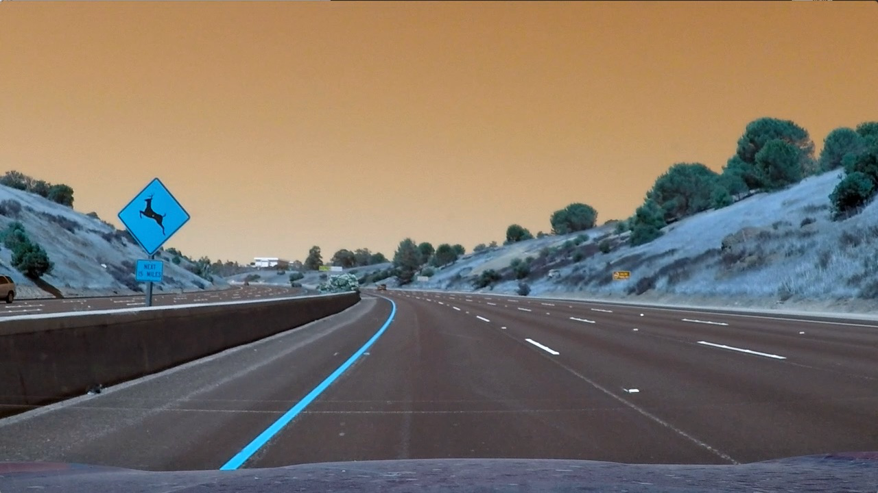
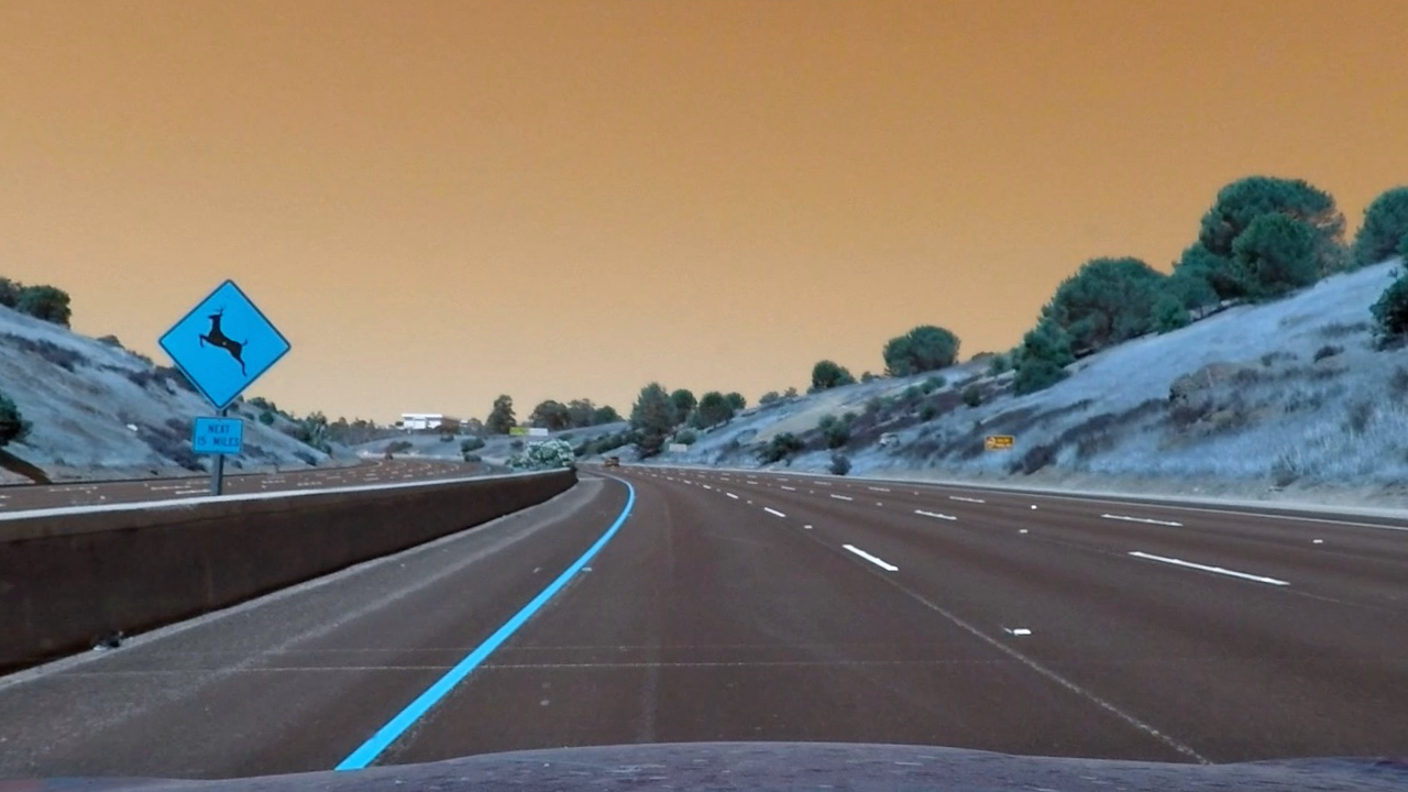
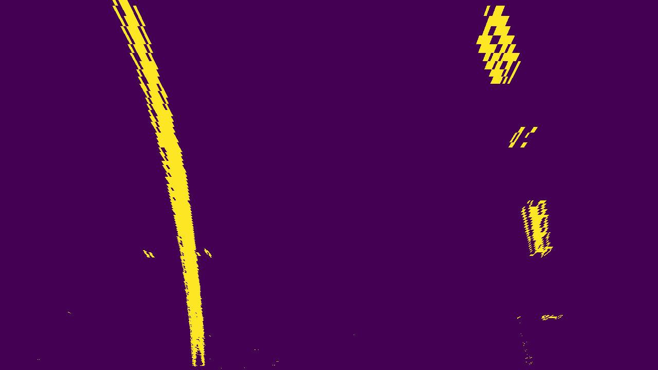
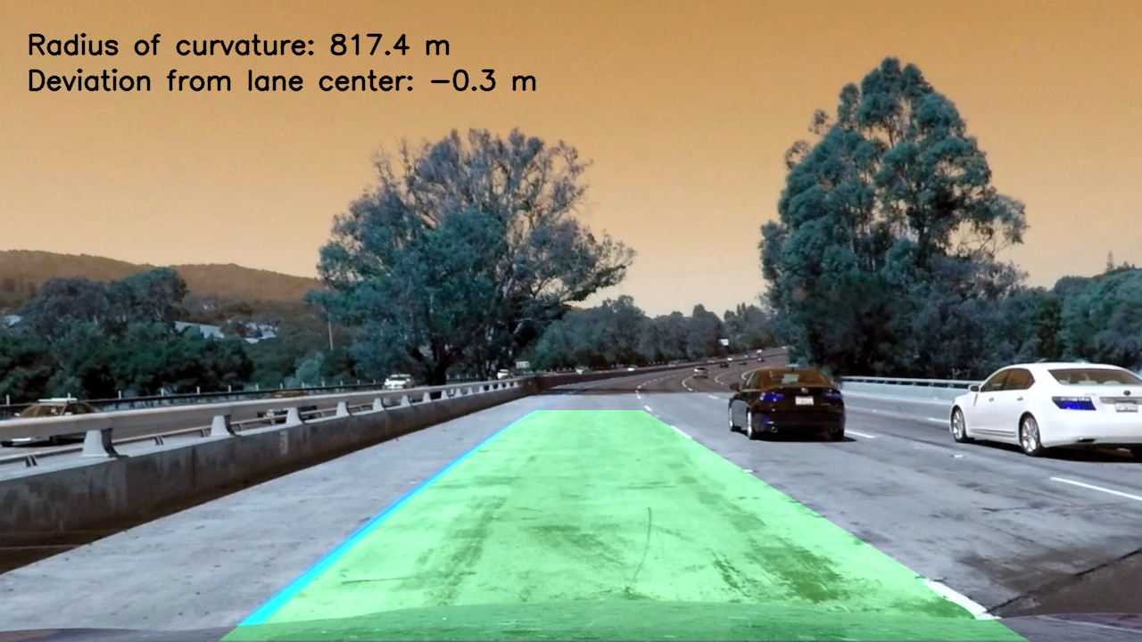
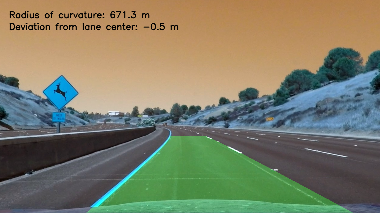
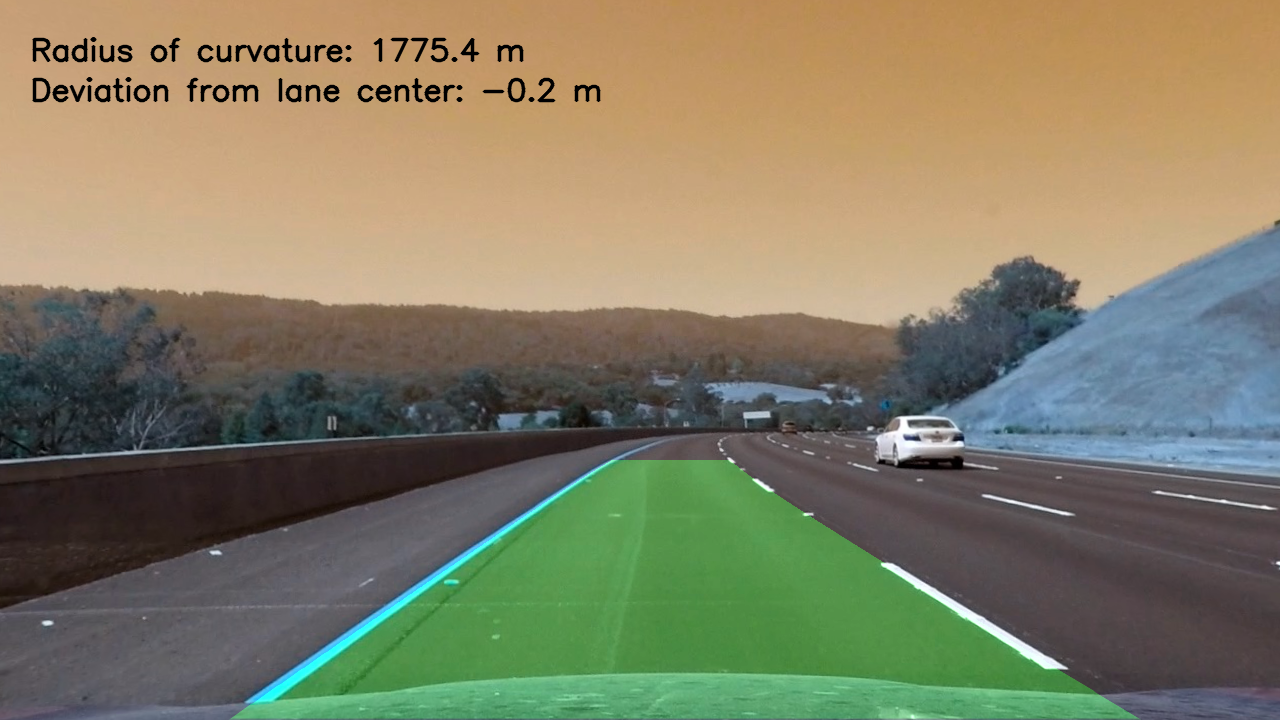
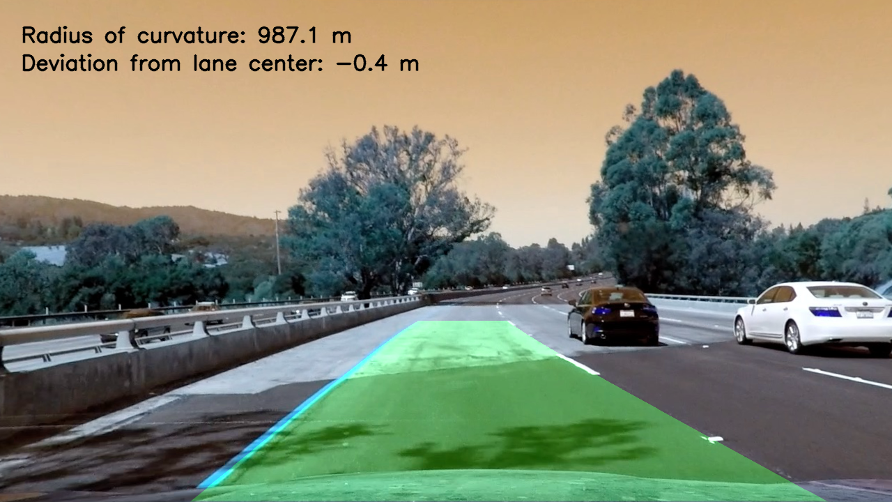
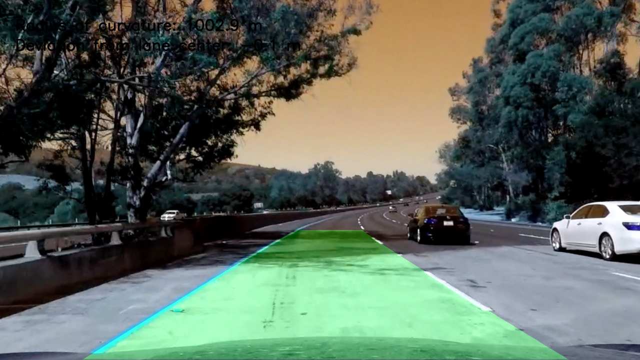
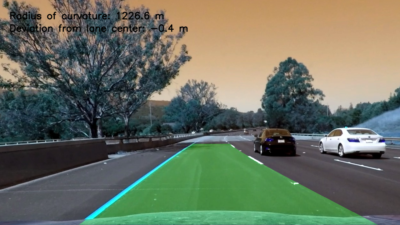
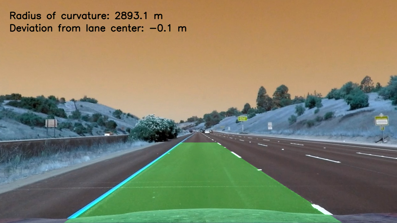
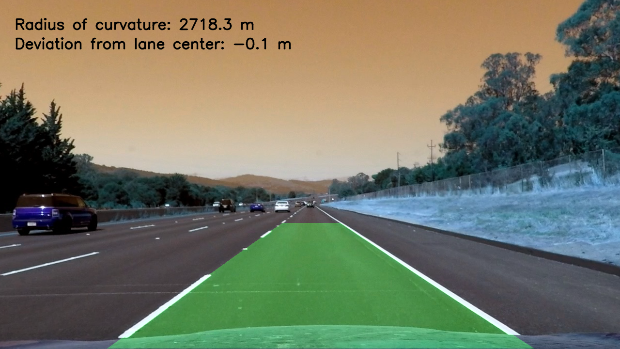
Advanced-lane-lines-finding-on-the-road: A Jupyter Notebook repository from Jeanyvesbourdoncle

SW Pipeline to identify the lane boundaries ina video from a front-facing camera on a car

Dynamic Results of lanes line detection on the road on the trial track here.

The differents steps of the SW Pipeline are the following :

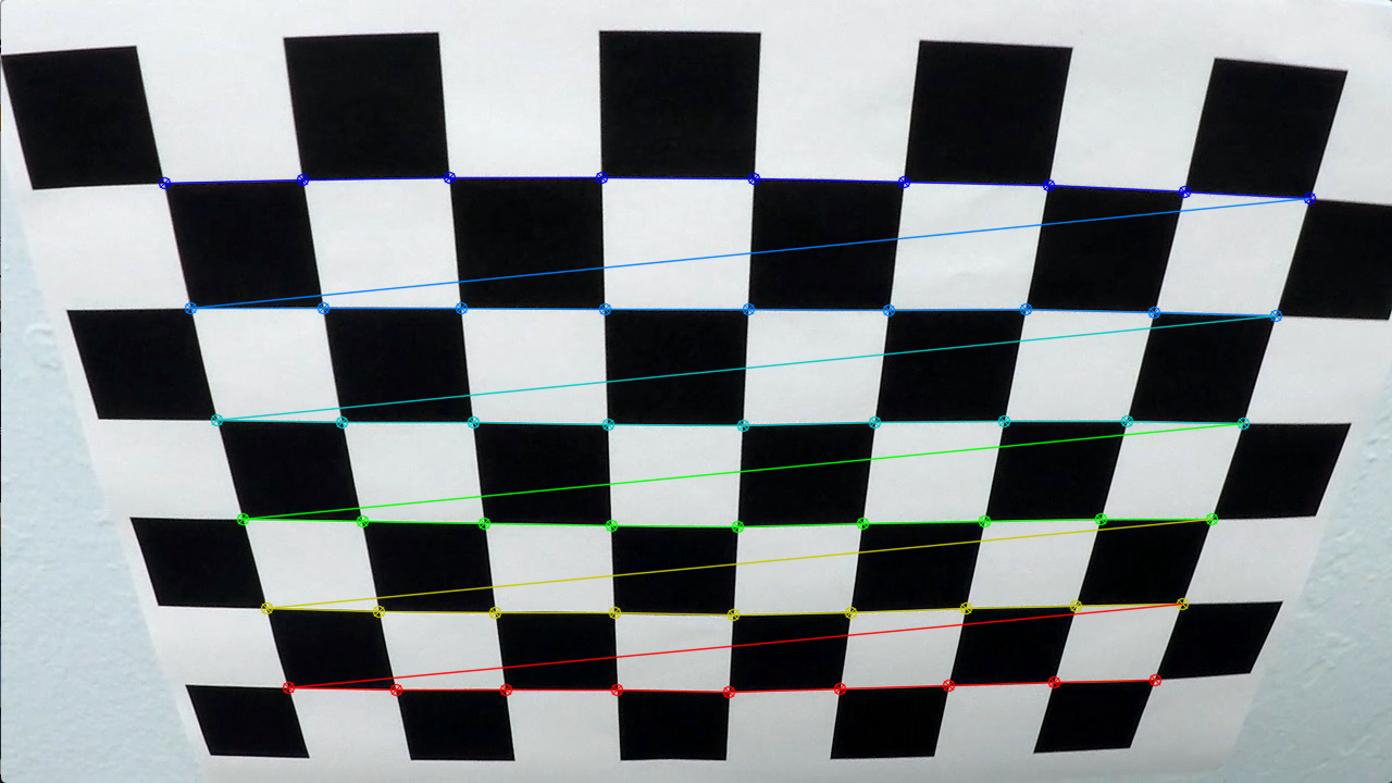
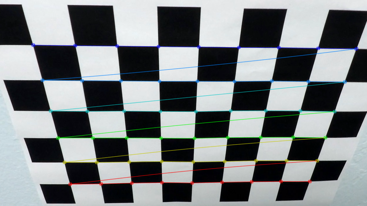
Step 0 : Compute the camera calibration matrix and distortion coefficients given a set of chessboard images.

Step 1 : Apply a distortion correction to raw images.

Step 2 : Use color transforms, gradients, etc., to create a thresholded binary image.

Step 3 : Apply a perspective transform to rectify binary image ("birds-eye view").

Step 4 : Detect lane pixels and fit to find the lane boundary.

Step 5 : Determine the curvature of the lane and vehicle position with respect to center. Warp the detected lane boundaries back onto the original image.

Step 6 : Output visual display of the lane boundaries and numerical estimation of lane curvature and vehicle position.

Program modularity

The generic fonctions are present in the module CV_function.py

This part is a generic part (must be not change).

Only a specific part is here present in this generic part:

modification of the differents threshold gradient (-x, -x, -mag, -dir) and threshold colors
modification of the 3 hyperparameters "window" (pixel analyze)

The main program is named SW_Pipeline_Advanced_Lane_Finding.ipynb

You can find in the other part named is named SW_Pipeline_Advanced_Lane_Finding.ipynb.

He calls for every stages of the SW pipeline the generic fonctionc impemented in the module CV_funtion.py

Step 0 : Camera Calibration

The functionnalities "camera calibration" and "distorsion correction" with the chessboards are directly implemented in the CV_function.py for the generic part.

For the specific part, the code is implemented in SW_Pipeline_Advanced_Lane_Finding.ipynb.

The SW design method is very good explains in the code comments.

Step 1 : Distorsion Correction

The functionnality "distorsion correction" is generic and directly implemented in the CV_function.py.

This module is call in SW_Pipeline_Advanced_Lane_Finding.ipynb.

The input are the raw image. The output is the undistorded image.

Step 2 : Color Transforms and Gradients

The functionnality "color transform and gradient thresholding" is generic and directly implemented in the CV_function.py.

The input images are the images after distorsion correction. The output images are the images witht the configured threshold.

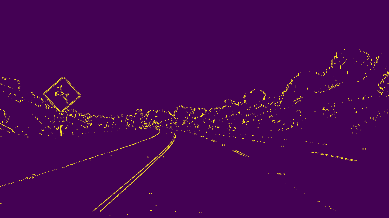
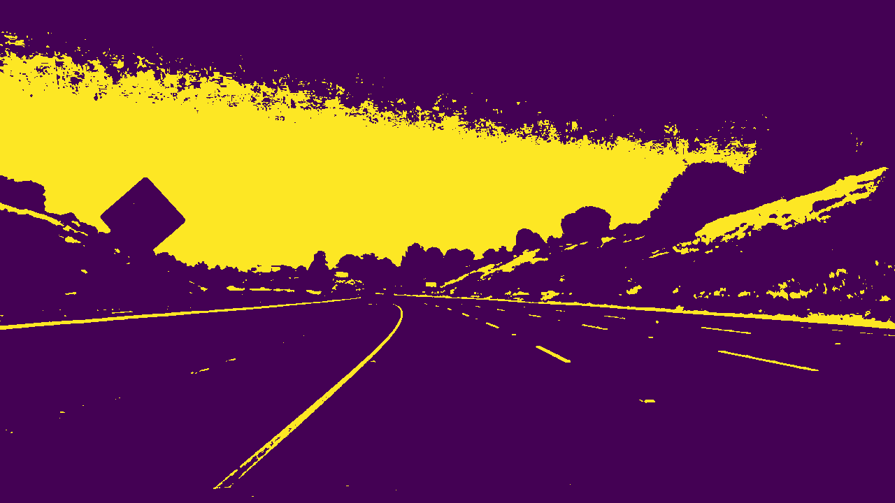
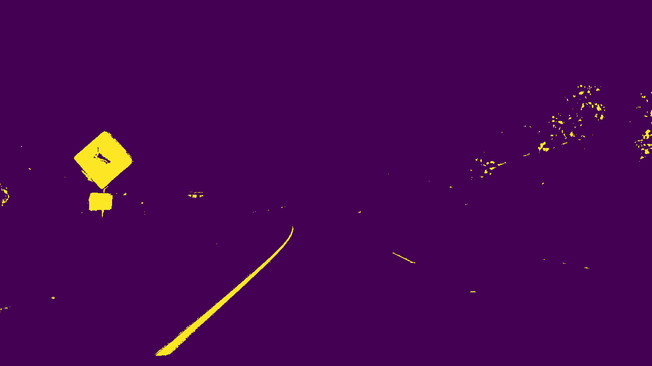
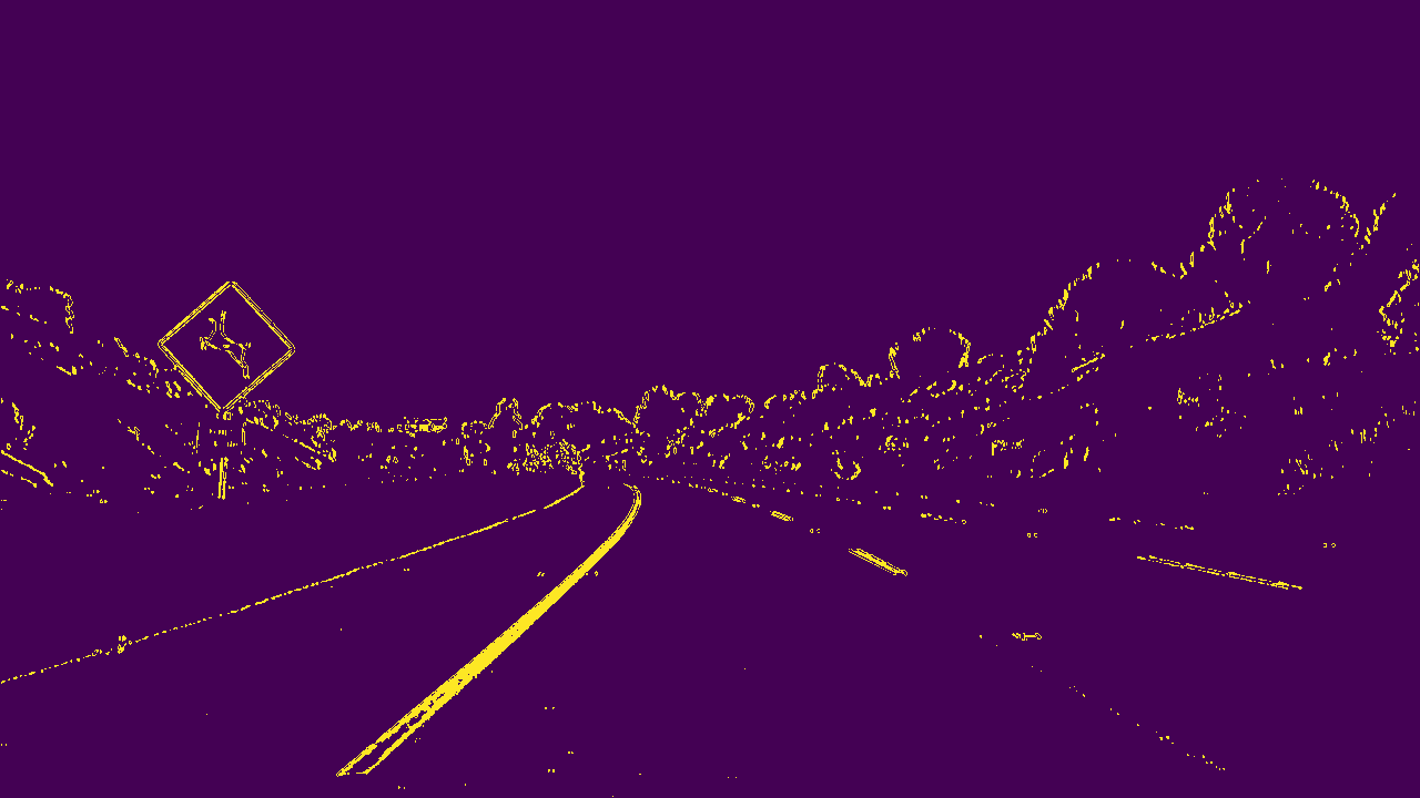
A lot of combinaison are possible (colors threshold/gradient-x/gradient-y/gradient direction/gradient magnitude). For this exercice, we used only the x-gradient and the colors transform (L+S Channel,L for the problem of shadow). The others parameters (mag/dir) have not been used.

This step (threshold configuration) costs a long time, because the thresholds are configured manually.

PLease find the 4 images bellow (with x-gradient thresholding alone, with thresholding color (S-Channel) alone, with thresholding color (L-Channel) alone and the combined solution)

Step 3 : Perspective Transform ("birds-eye view")

The functionnality "perspective transform" is generic and directly implemented in the CV_function.py.

The target is to take 4 points (x,y) very far in the image to make a better analyze and to make a perspective transform.

Step 4 : Lane line pixels and fit their positions with a polynomial

2 Steps are here useful :

the lane-line pixels identification and
the polynomial curve for every lane (right and left)

Two generics functionalities implemented in CV_function.py are here useful :

the lane-line pixel indentification and
the polynomial curve for every line.

For information : Blue and Red are the colors for the lane left and the lane right.

To add the two polynomial, these 2 lines are superposed on the plot with the 2 lanes pixels:

plt.plot(left_fitx, ploty, color='yellow')
plt.plot(right_fitx, ploty, color='yellow')

Step 5 : Calculation of the radius of curvature of the lane and the position of the vehicle with respect to center

We need 2 generics functionalities implemented in CV_function.py:

Step 1 : radius of curvature : The most important point is the transfert from the "pixel world" to the "real world" (in meters)

Step 2 : position of the vehicule

Step 6 : Main Program

Here you can find the pipeline with the comment (main programm) and the results for every frame :

####"PIPELINE"#### def process_image(image):

#Step 1 = camera calibration + image undistorted 
undist =calculation_undistort(image,objpoints,imgpoints)

#Step 2 = Threshold (gradient (-x/-y/-mag/-dir) and color) configuration and threshold combinaison
_, _, _, _, _, combined_binary,_ = image_computing(undist)

#Step 3 = Perspective Transform, the target is to select 4 points very far in the image foe a better analyze
# This function returns Minv, because he will be use in the Step, in the reconstitution step
warped,Minv = warper(combined_binary, src, dst)

#Step 4 : the target is to know the dedicated pixels for the lane right and the lane left 
# the standard method named "peak/histogram" is used (convolution mathod not used) with windows configured with hyperparameters
leftx, lefty, rightx, righty,left_lane_inds, right_lane_inds = find_lanes_pixels(warped)

#Step 5a = polynomial fonction for the right and the left curve
left_fit, right_fit, ploty, left_fitx, right_fitx, out_img= fit_polynomial (warped, leftx, lefty, rightx, righty, left_lane_inds, right_lane_inds)

#Step 5b = Diagnostic information 1 : curvature calculation (space conversion : from "pixel" world to "meters" world)
left_radius_curve,right_radius_curve = calculation_curvature (leftx, lefty, rightx, righty)

#Step 5c = Diagnostic information 2 : deviation of the vehicle with the "central line" reference
vehicle_position = calculation_vehicle_position (undist, left_fit, right_fit)

#Step 6 = Vizualization of the image (before processing) with all the informations (diagnostics + lane detection tracking)
result = vizualization(undist, left_fit, right_fit, Minv, left_radius_curve, left_radius_curve, vehicle_position)
 
return result

Jeanyvesbourdoncle/Advanced-lane-lines-finding-on-the-road