Cellular omics such as single-cell genomics, proteomics, and microbiomics allow the characterization of tissue and microbial community composition, which can be compared between conditions to identify biological drivers. This strategy has been critical to unveiling markers of disease progression in conditions such as cancer and pathogen infections.
For cellular omic data, no method for differential variability analysis exists, and methods for differential composition analysis only take a few fundamental data properties into account. Here we introduce sccomp, a generalised method for differential composition and variability analyses capable of jointly modelling data count distribution, compositionality, group-specific variability, and proportion mean-variability association, while being robust to outliers.
sccomp is an extensive analysis framework that allows realistic data simulation and cross-study knowledge transfer. We demonstrate that mean-variability association is ubiquitous across technologies, highlighting the inadequacy of the very popular Dirichlet-multinomial modeling and providing essential principles for differential variability analysis.

Mangiola, Stefano, Alexandra J. Roth-Schulze, Marie Trussart, Enrique Zozaya-Valdés, Mengyao Ma, Zijie Gao, Alan F. Rubin, Terence P. Speed, Heejung Shim, and Anthony T. Papenfuss. 2023. “Sccomp: Robust Differential Composition and Variability Analysis for Single-Cell Data.” Proceedings of the National Academy of Sciences of the United States of America 120 (33): e2203828120. https://doi.org/10.1073/pnas.2203828120 PNAS - sccomp: Robust differential composition and variability analysis for single-cell data
sccomp tests differences in cell type proportions from single-cell
data. It is robust against outliers, it models continuous and discrete
factors, and capable of random-effect/intercept modelling.
- Complex linear models with continuous and categorical covariates
- Multilevel modelling, with population fixed and random effects/intercept
- Modelling data from counts
- Testing differences in cell-type proportionality
- Testing differences in cell-type specific variability
- Cell-type information share for variability adaptive shrinkage
- Testing differential variability
- Probabilistic outlier identification
- Cross-dataset learning (hyperpriors).
sccomp is based on cmdstanr which provides the latest version of
cmdstan the Bayesian modelling tool. cmdstanr is not on CRAN, so we
need to have 3 simple step process (that will be prompted to the user is
forgot).
- R installation of
sccomp - R installation of
cmdstanr cmdstanrcall tocmdstaninstallation
Bioconductor
if (!requireNamespace("BiocManager")) install.packages("BiocManager")

# Step 1
BiocManager::install("sccomp")

# Step 2
install.packages("cmdstanr", repos = c("https://stan-dev.r-universe.dev/", getOption("repos")))

# Step 3
cmdstanr::check_cmdstan_toolchain(fix = TRUE) # Just checking system setting
cmdstanr::install_cmdstan()
Github
# Step 1
devtools::install_github("MangiolaLaboratory/sccomp")

# Step 2
install.packages("cmdstanr", repos = c("https://stan-dev.r-universe.dev/", getOption("repos")))

# Step 3
cmdstanr::check_cmdstan_toolchain(fix = TRUE) # Just checking system setting
cmdstanr::install_cmdstan()| Function | Description |
|---|---|
sccomp_estimate |
Fit the model onto the data, and estimate the coefficients |
sccomp_remove_outliers |
Identify outliers probabilistically based on the model fit, and exclude them from the estimation |
sccomp_test |
Calculate the probability that the coefficients are outside the H0 interval (i.e. test_composition_above_logit_fold_change) |
sccomp_replicate |
Simulate data from the model, or part of the model |
sccomp_predict |
Predicts proportions, based on the model, or part of the model |
sccomp_remove_unwanted_variation |
Removes the variability for unwanted factors |
plot |
Plots summary plots to asses significance |
library(dplyr)
library(sccomp)
library(ggplot2)
library(forcats)
library(tidyr)
data("seurat_obj")
data("sce_obj")
data("counts_obj")
sccomp can model changes in composition and variability. By default,
the formula for variability is either ~1, which assumes that the
cell-group variability is independent of any covariate or
~ factor_of_interest, which assumes that the model is dependent on the
factor of interest only. The variability model must be a subset of the
model for composition.
Of the output table, the estimate columns start with the prefix c_
indicate composition, or with v_ indicate variability (when
formula_variability is set).
sccomp_result =
  sce_obj |>
  sccomp_estimate(
    formula_composition = ~ type,
    .sample =  sample,
    .cell_group = cell_group,
    cores = 1
  ) |>
  sccomp_remove_outliers(cores = 1) |> # Optional
sccomp_test()sccomp_result =
counts_obj |>
sccomp_estimate(
formula_composition = ~ type,
.sample = sample,
.cell_group = cell_group,
.count = count,
cores = 1, verbose = FALSE
) |>
sccomp_remove_outliers(cores = 1, verbose = FALSE) |> # Optional
sccomp_test()## Running standalone generated quantities after 1 MCMC chain, with 1 thread(s) per chain...
##
## Chain 1 finished in 0.0 seconds.
## Running standalone generated quantities after 1 MCMC chain, with 1 thread(s) per chain...
##
## Chain 1 finished in 0.0 seconds.
Here you see the results of the fit, the effects of the factor on composition and variability. You also can see the uncertainty around those effects.
The output is a tibble containing the Following columns
cell_group- The cell groups being tested.parameter- The parameter being estimated from the design matrix described by the inputformula_compositionandformula_variability.factor- The covariate factor in the formula, if applicable (e.g., not present for Intercept or contrasts).c_lower- Lower (2.5%) quantile of the posterior distribution for a composition (c) parameter.c_effect- Mean of the posterior distribution for a composition (c) parameter.c_upper- Upper (97.5%) quantile of the posterior distribution for a composition (c) parameter.c_pH0- Probability of the null hypothesis (no difference) for a composition (c). This is not a p-value.c_FDR- False-discovery rate of the null hypothesis for a composition (c).v_lower- Lower (2.5%) quantile of the posterior distribution for a variability (v) parameter.v_effect- Mean of the posterior distribution for a variability (v) parameter.v_upper- Upper (97.5%) quantile of the posterior distribution for a variability (v) parameter.v_pH0- Probability of the null hypothesis for a variability (v).v_FDR- False-discovery rate of the null hypothesis for a variability (v).count_data- Nested input count data.
sccomp_result## # A tibble: 72 × 14
## cell_group parameter factor c_lower c_effect c_upper c_pH0 c_FDR v_lower
## <chr> <chr> <chr> <dbl> <dbl> <dbl> <dbl> <dbl> <dbl>
## 1 B1 (Intercep… <NA> 0.981 1.13 1.28 0 0 -6.33
## 2 B1 typecancer type -1.15 -0.892 -0.646 0 0 NA
## 3 B2 (Intercep… <NA> 0.476 0.781 1.08 0 0 -5.64
## 4 B2 typecancer type -1.20 -0.779 -0.346 5.00e-4 4.55e-5 NA
## 5 B3 (Intercep… <NA> -0.614 -0.326 -0.0416 6.27e-2 5.89e-3 -6.83
## 6 B3 typecancer type -0.622 -0.219 0.196 2.83e-1 7.30e-2 NA
## 7 BM (Intercep… <NA> -1.25 -0.948 -0.667 0 0 -7.44
## 8 BM typecancer type -0.738 -0.340 0.0937 1.37e-1 4.42e-2 NA
## 9 CD4 1 (Intercep… <NA> 0.208 0.385 0.562 2.25e-3 1.30e-4 -6.75
## 10 CD4 1 typecancer type -0.0828 0.150 0.388 3.38e-1 9.76e-2 NA
## # ℹ 62 more rows
## # ℹ 5 more variables: v_effect <dbl>, v_upper <dbl>, v_pH0 <dbl>, v_FDR <dbl>,
## # count_data <list>
A plot of group proportions, faceted by groups. The blue boxplots represent the posterior predictive check. If the model is descriptively adequate for the data, the blue boxplots should roughly overlay the black boxplots, which represent the observed data. The outliers are coloured in red. A boxplot will be returned for every (discrete) covariate present in formula_composition. The colour coding represents the significant associations for composition and/or variability.
sccomp_result |>
  sccomp_boxplot(factor = "type")
## Loading model from cache...
## Running standalone generated quantities after 1 MCMC chain, with 1 thread(s) per chain...
##
## Chain 1 finished in 0.0 seconds.
## Joining with `by = join_by(cell_group, sample)`
## Joining with `by = join_by(cell_group, type)`
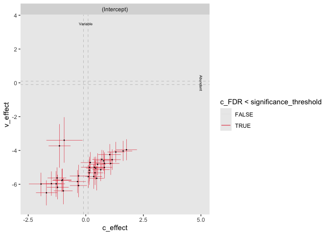
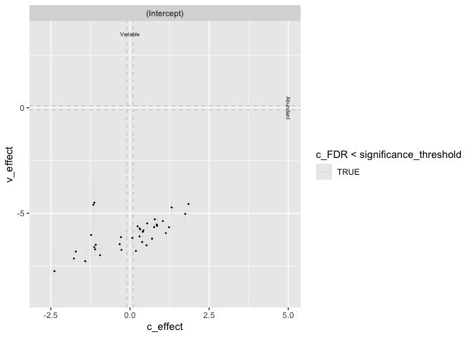
A plot of estimates of differential composition (c_) on the x-axis and differential variability (v_) on the y-axis. The error bars represent 95% credible intervals. The dashed lines represent the minimal effect that the hypothesis test is based on. An effect is labelled as significant if it exceeds the minimal effect according to the 95% credible interval. Facets represent the covariates in the model.
sccomp_result |>
  plot_1D_intervals()
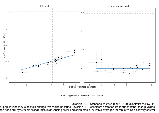
We can plot the relationship between abundance and variability. As we can see below, they are positively correlated. sccomp models this relationship to obtain a shrinkage effect on the estimates of both the abundance and the variability. This shrinkage is adaptive as it is modelled jointly, thanks to Bayesian inference.
sccomp_result |>
  plot_2D_intervals()
You can produce the series of plots calling the plot method.
sccomp_result |> plot() Note: If counts are available, we strongly discourage the use of proportions, as an important source of uncertainty (i.e., for rare groups/cell types) is not modeled.
The use of proportions is better suited for modelling deconvolution results (e.g., of bulk RNA data), in which case counts are not available.
Proportions should be greater than 0. Assuming that zeros derive from a precision threshold (e.g., deconvolution), zeros are converted to the smallest non-zero value.
sccomp is able to fit erbitrary complex models. In this example we
have a continuous and binary covariate.
res =
    seurat_obj |>
    sccomp_estimate(
      formula_composition = ~ type + continuous_covariate,
      .sample = sample, .cell_group = cell_group,
      cores = 1, verbose=FALSE
    )
## Loading required package: SeuratObject
## Loading required package: sp
##
## Attaching package: 'SeuratObject'
## The following objects are masked from 'package:base':
##
## intersect, t
## sccomp says: count column is an integer. The sum-constrained beta binomial model will be used
## sccomp says: estimation
## sccomp says: the composition design matrix has columns: (Intercept), typehealthy, continuous_covariate
## sccomp says: the variability design matrix has columns: (Intercept)
## Loading model from cache...
## sccomp says: to do hypothesis testing run `sccomp_test()`,
## the `test_composition_above_logit_fold_change` = 0.1 equates to a change of ~10%, and
## 0.7 equates to ~100% increase, if the baseline is ~0.1 proportion.
## Use `sccomp_proportional_fold_change` to convert c_effect (linear) to proportion difference (non-linear).
res## # A tibble: 90 × 10
## cell_group parameter factor c_lower c_effect c_upper v_lower v_effect v_upper
## <chr> <chr> <chr> <dbl> <dbl> <dbl> <dbl> <dbl> <dbl>
## 1 B immature (Interce… <NA> 0.377 0.759 1.12 -4.07 -3.67 -3.29
## 2 B immature typeheal… type 0.866 1.36 1.86 NA NA NA
## 3 B immature continuo… conti… -0.250 0.0610 0.378 NA NA NA
## 4 B mem (Interce… <NA> -1.25 -0.804 -0.365 -4.93 -4.52 -4.13
## 5 B mem typeheal… type 1.03 1.67 2.29 NA NA NA
## 6 B mem continuo… conti… -0.240 0.0896 0.415 NA NA NA
## 7 CD4 cm S1… (Interce… <NA> 1.17 1.49 1.82 -3.66 -3.27 -2.89
## 8 CD4 cm S1… typeheal… type 0.689 1.12 1.56 NA NA NA
## 9 CD4 cm S1… continuo… conti… -0.0662 0.187 0.441 NA NA NA
## 10 CD4 cm hi… (Interce… <NA> -0.940 -0.460 0.0176 -5.13 -4.63 -4.15
## # ℹ 80 more rows
## # ℹ 1 more variable: count_data <list>
sccomp supports multilevel modeling by allowing the inclusion of
random effects in the compositional and variability formulas. This is
particularly useful when your data has hierarchical or grouped
structures, such as measurements nested within subjects, batches, or
experimental units. By incorporating random effects, sccomp can account
for variability at different levels of your data, improving model fit
and inference accuracy.
In this example, we demonstrate how to fit a random intercept model using sccomp. We’ll model the cell-type proportions with both fixed effects (e.g., treatment) and random effects (e.g., subject-specific variability).
Here is the input data
seurat_obj[[]] |> as_tibble()## # A tibble: 106,297 × 9
## cell_group nCount_RNA nFeature_RNA group__ group__wrong sample type group2__
## <chr> <dbl> <int> <chr> <chr> <chr> <chr> <chr>
## 1 CD4 naive 0 0 GROUP1 1 SI-GA… canc… GROUP21
## 2 Mono clas… 0 0 GROUP1 1 SI-GA… canc… GROUP21
## 3 CD4 cm S1… 0 0 GROUP1 1 SI-GA… canc… GROUP21
## 4 B immature 0 0 GROUP1 1 SI-GA… canc… GROUP21
## 5 CD8 naive 0 0 GROUP1 1 SI-GA… canc… GROUP21
## 6 CD4 naive 0 0 GROUP1 1 SI-GA… canc… GROUP21
## 7 Mono clas… 0 0 GROUP1 1 SI-GA… canc… GROUP21
## 8 CD4 cm S1… 0 0 GROUP1 1 SI-GA… canc… GROUP21
## 9 CD4 cm hi… 0 0 GROUP1 1 SI-GA… canc… GROUP21
## 10 B immature 0 0 GROUP1 1 SI-GA… canc… GROUP21
## # ℹ 106,287 more rows
## # ℹ 1 more variable: continuous_covariate <dbl>
res =
  seurat_obj |>
  sccomp_estimate(
    formula_composition = ~ type + (1 | group__),
    .sample = sample,
    .cell_group = cell_group,
    bimodal_mean_variability_association = TRUE,
    cores = 1, verbose = FALSE
  )
## sccomp says: count column is an integer. The sum-constrained beta binomial model will be used
## sccomp says: estimation
## sccomp says: the composition design matrix has columns: (Intercept), typehealthy
## sccomp says: the variability design matrix has columns: (Intercept)
## Loading model from cache...
## sccomp says: to do hypothesis testing run `sccomp_test()`,
## the `test_composition_above_logit_fold_change` = 0.1 equates to a change of ~10%, and
## 0.7 equates to ~100% increase, if the baseline is ~0.1 proportion.
## Use `sccomp_proportional_fold_change` to convert c_effect (linear) to proportion difference (non-linear).
res## # A tibble: 180 × 10
## cell_group parameter factor c_lower c_effect c_upper v_lower v_effect v_upper
## <chr> <chr> <chr> <dbl> <dbl> <dbl> <dbl> <dbl> <dbl>
## 1 B immature (Interce… <NA> 0.498 0.839 1.17 -4.09 -3.66 -3.14
## 2 B immature typeheal… type 0.687 1.08 1.53 NA NA NA
## 3 B immature (Interce… <NA> -0.324 0.0821 0.672 NA NA NA
## 4 B immature (Interce… <NA> -0.0712 0.276 0.796 NA NA NA
## 5 B immature (Interce… <NA> -0.183 0.204 0.636 NA NA NA
## 6 B immature (Interce… <NA> -0.744 -0.311 0.0402 NA NA NA
## 7 B mem (Interce… <NA> -0.769 -0.281 0.133 -4.96 -4.44 -3.88
## 8 B mem typeheal… type 0.309 0.959 1.63 NA NA NA
## 9 B mem (Interce… <NA> -0.294 0.0881 0.679 NA NA NA
## 10 B mem (Interce… <NA> -0.0411 0.335 0.907 NA NA NA
## # ℹ 170 more rows
## # ℹ 1 more variable: count_data <list>
sccomp can model random slopes. We providean example below.
res =
  seurat_obj |>
  sccomp_estimate(
      formula_composition = ~ type + (type | group__),
      .sample = sample,
      .cell_group = cell_group,
      bimodal_mean_variability_association = TRUE,
      cores = 1, verbose = FALSE
    )
## sccomp says: count column is an integer. The sum-constrained beta binomial model will be used
## sccomp says: estimation
## sccomp says: the composition design matrix has columns: (Intercept), typehealthy
## sccomp says: the variability design matrix has columns: (Intercept)
## Loading model from cache...
## sccomp says: to do hypothesis testing run `sccomp_test()`,
## the `test_composition_above_logit_fold_change` = 0.1 equates to a change of ~10%, and
## 0.7 equates to ~100% increase, if the baseline is ~0.1 proportion.
## Use `sccomp_proportional_fold_change` to convert c_effect (linear) to proportion difference (non-linear).
res## # A tibble: 240 × 10
## cell_group parameter factor c_lower c_effect c_upper v_lower v_effect v_upper
## <chr> <chr> <chr> <dbl> <dbl> <dbl> <dbl> <dbl> <dbl>
## 1 B immature (Interce… <NA> 0.489 0.848 1.29 -4.17 -3.67 -2.97
## 2 B immature typeheal… type 0.490 1.03 1.51 NA NA NA
## 3 B immature (Interce… <NA> -0.186 0.0634 0.523 NA NA NA
## 4 B immature typeheal… <NA> -0.215 0.0533 0.494 NA NA NA
## 5 B immature (Interce… <NA> -0.195 0.142 0.607 NA NA NA
## 6 B immature typeheal… <NA> -0.159 0.144 0.582 NA NA NA
## 7 B immature (Interce… <NA> -0.148 0.176 0.611 NA NA NA
## 8 B immature (Interce… <NA> -0.752 -0.269 0.0267 NA NA NA
## 9 B mem (Interce… <NA> -0.738 -0.331 0.0703 -4.97 -4.42 -3.78
## 10 B mem typeheal… type 0.317 0.923 1.58 NA NA NA
## # ℹ 230 more rows
## # ℹ 1 more variable: count_data <list>
If you have a more complex hierarchy, such as measurements nested within
subjects and subjects nested within batches, you can include multiple
grouping variables. Here group2__ is nested within group__.
res =
  seurat_obj |>
  sccomp_estimate(
      formula_composition = ~ type + (type | group__) + (1 | group2__),
      .sample = sample,
      .cell_group = cell_group,
      bimodal_mean_variability_association = TRUE,
      cores = 1, verbose = FALSE
    )
## sccomp says: count column is an integer. The sum-constrained beta binomial model will be used
## sccomp says: estimation
## sccomp says: the composition design matrix has columns: (Intercept), typehealthy
## sccomp says: the variability design matrix has columns: (Intercept)
## Loading model from cache...
## sccomp says: to do hypothesis testing run `sccomp_test()`,
## the `test_composition_above_logit_fold_change` = 0.1 equates to a change of ~10%, and
## 0.7 equates to ~100% increase, if the baseline is ~0.1 proportion.
## Use `sccomp_proportional_fold_change` to convert c_effect (linear) to proportion difference (non-linear).
res## # A tibble: 300 × 10
## cell_group parameter factor c_lower c_effect c_upper v_lower v_effect v_upper
## <chr> <chr> <chr> <dbl> <dbl> <dbl> <dbl> <dbl> <dbl>
## 1 B immature (Interce… <NA> 0.437 0.820 1.27 -4.28 -3.63 -2.94
## 2 B immature typeheal… type 0.700 1.13 1.67 NA NA NA
## 3 B immature (Interce… <NA> -0.202 0.0312 0.550 NA NA NA
## 4 B immature typeheal… <NA> -0.158 0.0252 0.446 NA NA NA
## 5 B immature (Interce… <NA> -0.192 0.0614 0.365 NA NA NA
## 6 B immature typeheal… <NA> -0.130 0.0555 0.349 NA NA NA
## 7 B immature (Interce… <NA> -0.106 0.105 0.534 NA NA NA
## 8 B immature (Interce… <NA> -0.712 -0.150 0.0377 NA NA NA
## 9 B immature (Interce… <NA> -0.407 -0.0769 0.0888 NA NA NA
## 10 B immature (Interce… <NA> -0.0716 0.133 0.609 NA NA NA
## # ℹ 290 more rows
## # ℹ 1 more variable: count_data <list>
The estimated effects are expressed in the unconstrained space of the parameters, similar to differential expression analysis that expresses changes in terms of log fold change. However, for differences in proportion, logit fold change must be used, which is harder to interpret and understand.
Therefore, we provide a more intuitive proportional fold change that can be more easily understood. However, these cannot be used to infer significance (use sccomp_test() instead), and a lot of care must be taken given the nonlinearity of these measures (a 1-fold increase from 0.0001 to 0.0002 carries a different weight than a 1-fold increase from 0.4 to 0.8).
From your estimates, you can specify which effects you are interested in (this can be a subset of the full model if you wish to exclude unwanted effects), and the two points you would like to compare.
In the case of a categorical variable, the starting and ending points are categories.
sccomp_result |>
   sccomp_proportional_fold_change(
     formula_composition = ~  type,
     from =  "healthy",
     to = "cancer"
    ) |>
  select(cell_group, statement)
## Loading model from cache...
## Running standalone generated quantities after 1 MCMC chain, with 1 thread(s) per chain...
##
## Chain 1 finished in 0.0 seconds.
## # A tibble: 36 × 2
## cell_group statement
## <chr> <glue>
## 1 B1 2.4-fold decrease (from 0.0541 to 0.0223)
## 2 B2 2.2-fold decrease (from 0.0382 to 0.0177)
## 3 B3 1.3-fold decrease (from 0.0129 to 0.0102)
## 4 BM 1.4-fold decrease (from 0.0068 to 0.0049)
## 5 CD4 1 1.1-fold increase (from 0.0258 to 0.0296)
## 6 CD4 2 1.7-fold increase (from 0.0498 to 0.0828)
## 7 CD4 3 3.4-fold decrease (from 0.1111 to 0.0327)
## 8 CD4 4 1.2-fold increase (from 0.0017 to 0.002)
## 9 CD4 5 1.1-fold increase (from 0.0305 to 0.0325)
## 10 CD8 1 1.3-fold increase (from 0.1 to 0.1254)
## # ℹ 26 more rows
seurat_obj |>
  sccomp_estimate(
    formula_composition = ~ 0 + type,
    .sample = sample,
    .cell_group = cell_group,
    cores = 1, verbose = FALSE
  ) |>
  sccomp_test( contrasts =  c("typecancer - typehealthy", "typehealthy - typecancer"))
## # A tibble: 60 × 14
## cell_group parameter factor c_lower c_effect c_upper c_pH0 c_FDR v_lower
## <chr> <chr> <chr> <dbl> <dbl> <dbl> <dbl> <dbl> <dbl>
## 1 B immature typecanc… <NA> -1.89 -1.35 -0.803 0 0 NA
## 2 B immature typeheal… <NA> 0.803 1.35 1.89 0 0 NA
## 3 B mem typecanc… <NA> -2.26 -1.64 -1.04 0 0 NA
## 4 B mem typeheal… <NA> 1.04 1.64 2.26 0 0 NA
## 5 CD4 cm S10… typecanc… <NA> -1.43 -0.993 -0.531 0 0 NA
## 6 CD4 cm S10… typeheal… <NA> 0.531 0.993 1.43 0 0 NA
## 7 CD4 cm hig… typecanc… <NA> 0.847 1.56 2.24 0 0 NA
## 8 CD4 cm hig… typeheal… <NA> -2.24 -1.56 -0.847 0 0 NA
## 9 CD4 cm rib… typecanc… <NA> 0.264 0.931 1.57 0.00750 0.00180 NA
## 10 CD4 cm rib… typeheal… <NA> -1.57 -0.931 -0.264 0.00750 0.00180 NA
## # ℹ 50 more rows
## # ℹ 5 more variables: v_effect <dbl>, v_upper <dbl>, v_pH0 <dbl>, v_FDR <dbl>,
## # count_data <list>
This is achieved through model comparison with loo. In the following
example, the model with association with factors better fits the data
compared to the baseline model with no factor association. For
comparisons check_outliers must be set to FALSE as the leave-one-out
must work with the same amount of data, while outlier elimination does
not guarantee it.
If elpd_diff is away from zero of > 5 se_diff difference of 5, we
are confident that a model is better than the other
reference.
In this case, -79.9 / 11.5 = -6.9, therefore we can conclude that model
one, the one with factor association, is better than model two.
library(loo)

# Fit first model
model_with_factor_association =
  seurat_obj |>
  sccomp_estimate(
    formula_composition = ~ type,
    .sample =  sample,
    .cell_group = cell_group,
    inference_method = "hmc",
    enable_loo = TRUE
  )
## Running MCMC with 6 parallel chains, with 3 thread(s) per chain...
##
## Chain 1 Iteration: 1 / 966 [ 0%] (Warmup)
## Chain 1 Iteration: 100 / 966 [ 10%] (Warmup)
## Chain 1 Iteration: 200 / 966 [ 20%] (Warmup)
## Chain 2 Iteration: 1 / 966 [ 0%] (Warmup)
## Chain 2 Iteration: 100 / 966 [ 10%] (Warmup)
## Chain 3 Iteration: 1 / 966 [ 0%] (Warmup)
## Chain 3 Iteration: 100 / 966 [ 10%] (Warmup)
## Chain 4 Iteration: 1 / 966 [ 0%] (Warmup)
## Chain 4 Iteration: 100 / 966 [ 10%] (Warmup)
## Chain 5 Iteration: 1 / 966 [ 0%] (Warmup)
## Chain 6 Iteration: 1 / 966 [ 0%] (Warmup)
## Chain 1 Iteration: 300 / 966 [ 31%] (Warmup)
## Chain 1 Iteration: 301 / 966 [ 31%] (Sampling)
## Chain 2 Iteration: 200 / 966 [ 20%] (Warmup)
## Chain 3 Iteration: 200 / 966 [ 20%] (Warmup)
## Chain 1 Iteration: 400 / 966 [ 41%] (Sampling)
## Chain 2 Iteration: 300 / 966 [ 31%] (Warmup)
## Chain 2 Iteration: 301 / 966 [ 31%] (Sampling)
## Chain 4 Iteration: 200 / 966 [ 20%] (Warmup)
## Chain 5 Iteration: 100 / 966 [ 10%] (Warmup)
## Chain 6 Iteration: 100 / 966 [ 10%] (Warmup)
## Chain 3 Iteration: 300 / 966 [ 31%] (Warmup)
## Chain 3 Iteration: 301 / 966 [ 31%] (Sampling)
## Chain 2 Iteration: 400 / 966 [ 41%] (Sampling)
## Chain 4 Iteration: 300 / 966 [ 31%] (Warmup)
## Chain 4 Iteration: 301 / 966 [ 31%] (Sampling)
## Chain 5 Iteration: 200 / 966 [ 20%] (Warmup)
## Chain 1 Iteration: 500 / 966 [ 51%] (Sampling)
## Chain 3 Iteration: 400 / 966 [ 41%] (Sampling)
## Chain 6 Iteration: 200 / 966 [ 20%] (Warmup)
## Chain 4 Iteration: 400 / 966 [ 41%] (Sampling)
## Chain 5 Iteration: 300 / 966 [ 31%] (Warmup)
## Chain 5 Iteration: 301 / 966 [ 31%] (Sampling)
## Chain 1 Iteration: 600 / 966 [ 62%] (Sampling)
## Chain 2 Iteration: 500 / 966 [ 51%] (Sampling)
## Chain 6 Iteration: 300 / 966 [ 31%] (Warmup)
## Chain 6 Iteration: 301 / 966 [ 31%] (Sampling)
## Chain 3 Iteration: 500 / 966 [ 51%] (Sampling)
## Chain 4 Iteration: 500 / 966 [ 51%] (Sampling)
## Chain 5 Iteration: 400 / 966 [ 41%] (Sampling)
## Chain 1 Iteration: 700 / 966 [ 72%] (Sampling)
## Chain 2 Iteration: 600 / 966 [ 62%] (Sampling)
## Chain 6 Iteration: 400 / 966 [ 41%] (Sampling)
## Chain 3 Iteration: 600 / 966 [ 62%] (Sampling)
## Chain 5 Iteration: 500 / 966 [ 51%] (Sampling)
## Chain 2 Iteration: 700 / 966 [ 72%] (Sampling)
## Chain 4 Iteration: 600 / 966 [ 62%] (Sampling)
## Chain 1 Iteration: 800 / 966 [ 82%] (Sampling)
## Chain 3 Iteration: 700 / 966 [ 72%] (Sampling)
## Chain 6 Iteration: 500 / 966 [ 51%] (Sampling)
## Chain 2 Iteration: 800 / 966 [ 82%] (Sampling)
## Chain 4 Iteration: 700 / 966 [ 72%] (Sampling)
## Chain 5 Iteration: 600 / 966 [ 62%] (Sampling)
## Chain 1 Iteration: 900 / 966 [ 93%] (Sampling)
## Chain 3 Iteration: 800 / 966 [ 82%] (Sampling)
## Chain 6 Iteration: 600 / 966 [ 62%] (Sampling)
## Chain 2 Iteration: 900 / 966 [ 93%] (Sampling)
## Chain 4 Iteration: 800 / 966 [ 82%] (Sampling)
## Chain 5 Iteration: 700 / 966 [ 72%] (Sampling)
## Chain 1 Iteration: 966 / 966 [100%] (Sampling)
## Chain 3 Iteration: 900 / 966 [ 93%] (Sampling)
## Chain 6 Iteration: 700 / 966 [ 72%] (Sampling)
## Chain 1 finished in 2.3 seconds.
## Chain 2 Iteration: 966 / 966 [100%] (Sampling)
## Chain 4 Iteration: 900 / 966 [ 93%] (Sampling)
## Chain 5 Iteration: 800 / 966 [ 82%] (Sampling)
## Chain 2 finished in 2.3 seconds.
## Chain 3 Iteration: 966 / 966 [100%] (Sampling)
## Chain 4 Iteration: 966 / 966 [100%] (Sampling)
## Chain 3 finished in 2.3 seconds.
## Chain 4 finished in 2.3 seconds.
## Chain 5 Iteration: 900 / 966 [ 93%] (Sampling)
## Chain 6 Iteration: 800 / 966 [ 82%] (Sampling)
## Chain 5 Iteration: 966 / 966 [100%] (Sampling)
## Chain 5 finished in 2.4 seconds.
## Chain 6 Iteration: 900 / 966 [ 93%] (Sampling)
## Chain 6 Iteration: 966 / 966 [100%] (Sampling)
## Chain 6 finished in 2.5 seconds.
##
## All 6 chains finished successfully.
## Mean chain execution time: 2.4 seconds.
## Total execution time: 3.2 seconds.
# Fit second model
model_without_association =
  seurat_obj |>
  sccomp_estimate(
    formula_composition = ~ 1,
    .sample =  sample,
    .cell_group = cell_group,
    inference_method = "hmc",
    enable_loo = TRUE
  )
## Running MCMC with 6 parallel chains, with 3 thread(s) per chain...
##
## Chain 1 Iteration: 1 / 966 [ 0%] (Warmup)
## Chain 1 Iteration: 100 / 966 [ 10%] (Warmup)
## Chain 1 Iteration: 200 / 966 [ 20%] (Warmup)
## Chain 2 Iteration: 1 / 966 [ 0%] (Warmup)
## Chain 2 Iteration: 100 / 966 [ 10%] (Warmup)
## Chain 2 Iteration: 200 / 966 [ 20%] (Warmup)
## Chain 3 Iteration: 1 / 966 [ 0%] (Warmup)
## Chain 3 Iteration: 100 / 966 [ 10%] (Warmup)
## Chain 4 Iteration: 1 / 966 [ 0%] (Warmup)
## Chain 4 Iteration: 100 / 966 [ 10%] (Warmup)
## Chain 5 Iteration: 1 / 966 [ 0%] (Warmup)
## Chain 6 Iteration: 1 / 966 [ 0%] (Warmup)
## Chain 1 Iteration: 300 / 966 [ 31%] (Warmup)
## Chain 1 Iteration: 301 / 966 [ 31%] (Sampling)
## Chain 3 Iteration: 200 / 966 [ 20%] (Warmup)
## Chain 5 Iteration: 100 / 966 [ 10%] (Warmup)
## Chain 2 Iteration: 300 / 966 [ 31%] (Warmup)
## Chain 2 Iteration: 301 / 966 [ 31%] (Sampling)
## Chain 4 Iteration: 200 / 966 [ 20%] (Warmup)
## Chain 6 Iteration: 100 / 966 [ 10%] (Warmup)
## Chain 1 Iteration: 400 / 966 [ 41%] (Sampling)
## Chain 3 Iteration: 300 / 966 [ 31%] (Warmup)
## Chain 3 Iteration: 301 / 966 [ 31%] (Sampling)
## Chain 5 Iteration: 200 / 966 [ 20%] (Warmup)
## Chain 2 Iteration: 400 / 966 [ 41%] (Sampling)
## Chain 4 Iteration: 300 / 966 [ 31%] (Warmup)
## Chain 4 Iteration: 301 / 966 [ 31%] (Sampling)
## Chain 6 Iteration: 200 / 966 [ 20%] (Warmup)
## Chain 1 Iteration: 500 / 966 [ 51%] (Sampling)
## Chain 3 Iteration: 400 / 966 [ 41%] (Sampling)
## Chain 5 Iteration: 300 / 966 [ 31%] (Warmup)
## Chain 5 Iteration: 301 / 966 [ 31%] (Sampling)
## Chain 2 Iteration: 500 / 966 [ 51%] (Sampling)
## Chain 4 Iteration: 400 / 966 [ 41%] (Sampling)
## Chain 6 Iteration: 300 / 966 [ 31%] (Warmup)
## Chain 6 Iteration: 301 / 966 [ 31%] (Sampling)
## Chain 3 Iteration: 500 / 966 [ 51%] (Sampling)
## Chain 5 Iteration: 400 / 966 [ 41%] (Sampling)
## Chain 1 Iteration: 600 / 966 [ 62%] (Sampling)
## Chain 2 Iteration: 600 / 966 [ 62%] (Sampling)
## Chain 4 Iteration: 500 / 966 [ 51%] (Sampling)
## Chain 6 Iteration: 400 / 966 [ 41%] (Sampling)
## Chain 3 Iteration: 600 / 966 [ 62%] (Sampling)
## Chain 1 Iteration: 700 / 966 [ 72%] (Sampling)
## Chain 4 Iteration: 600 / 966 [ 62%] (Sampling)
## Chain 5 Iteration: 500 / 966 [ 51%] (Sampling)
## Chain 2 Iteration: 700 / 966 [ 72%] (Sampling)
## Chain 6 Iteration: 500 / 966 [ 51%] (Sampling)
## Chain 1 Iteration: 800 / 966 [ 82%] (Sampling)
## Chain 3 Iteration: 700 / 966 [ 72%] (Sampling)
## Chain 4 Iteration: 700 / 966 [ 72%] (Sampling)
## Chain 5 Iteration: 600 / 966 [ 62%] (Sampling)
## Chain 2 Iteration: 800 / 966 [ 82%] (Sampling)
## Chain 6 Iteration: 600 / 966 [ 62%] (Sampling)
## Chain 3 Iteration: 800 / 966 [ 82%] (Sampling)
## Chain 4 Iteration: 800 / 966 [ 82%] (Sampling)
## Chain 5 Iteration: 700 / 966 [ 72%] (Sampling)
## Chain 1 Iteration: 900 / 966 [ 93%] (Sampling)
## Chain 2 Iteration: 900 / 966 [ 93%] (Sampling)
## Chain 6 Iteration: 700 / 966 [ 72%] (Sampling)
## Chain 1 Iteration: 966 / 966 [100%] (Sampling)
## Chain 3 Iteration: 900 / 966 [ 93%] (Sampling)
## Chain 4 Iteration: 900 / 966 [ 93%] (Sampling)
## Chain 5 Iteration: 800 / 966 [ 82%] (Sampling)
## Chain 1 finished in 2.4 seconds.
## Chain 2 Iteration: 966 / 966 [100%] (Sampling)
## Chain 3 Iteration: 966 / 966 [100%] (Sampling)
## Chain 6 Iteration: 800 / 966 [ 82%] (Sampling)
## Chain 2 finished in 2.3 seconds.
## Chain 3 finished in 2.3 seconds.
## Chain 4 Iteration: 966 / 966 [100%] (Sampling)
## Chain 5 Iteration: 900 / 966 [ 93%] (Sampling)
## Chain 4 finished in 2.2 seconds.
## Chain 6 Iteration: 900 / 966 [ 93%] (Sampling)
## Chain 5 Iteration: 966 / 966 [100%] (Sampling)
## Chain 5 finished in 2.3 seconds.
## Chain 6 Iteration: 966 / 966 [100%] (Sampling)
## Chain 6 finished in 2.3 seconds.
##
## All 6 chains finished successfully.
## Mean chain execution time: 2.3 seconds.
## Total execution time: 3.0 seconds.
# Compare models
loo_compare(
   attr(model_with_factor_association, "fit")$loo(),
   attr(model_without_association, "fit")$loo()
)
## elpd_diff se_diff
## model1 0.0 0.0
## model2 -79.5 10.7
We can model the cell-group variability also dependent on the type, and so test differences in variability
res =
  seurat_obj |>
  sccomp_estimate(
    formula_composition = ~ type,
    formula_variability = ~ type,
    .sample = sample,
    .cell_group = cell_group,
    cores = 1, verbose = FALSE
  )

res
## # A tibble: 60 × 10
## cell_group parameter factor c_lower c_effect c_upper v_lower v_effect
## <chr> <chr> <chr> <dbl> <dbl> <dbl> <dbl> <dbl>
## 1 B immature (Interce… <NA> 0.330 0.748 1.15 -4.36 -3.95
## 2 B immature typeheal… type 0.815 1.36 1.89 -0.871 -0.224
## 3 B mem (Interce… <NA> -1.34 -0.864 -0.368 -5.14 -4.65
## 4 B mem typeheal… type 1.08 1.72 2.36 -1.41 -0.683
## 5 CD4 cm S100A4 (Interce… <NA> 1.33 1.67 2.01 -3.79 -3.40
## 6 CD4 cm S100A4 typeheal… type 0.387 0.835 1.28 -1.19 -0.687
## 7 CD4 cm high cytok… (Interce… <NA> -1.03 -0.511 0.0200 -5.13 -4.62
## 8 CD4 cm high cytok… typeheal… type -1.91 -1.08 -0.144 0.477 1.31
## 9 CD4 cm ribosome (Interce… <NA> -0.152 0.330 0.816 -4.90 -4.38
## 10 CD4 cm ribosome typeheal… type -1.74 -1.06 -0.393 -0.357 0.261
## # ℹ 50 more rows
## # ℹ 2 more variables: v_upper <dbl>, count_data <list>
Plot 1D significance plot
plots = res |> sccomp_test() |> plot()## Loading model from cache...
## Running standalone generated quantities after 1 MCMC chain, with 1 thread(s) per chain...
##
## Chain 1 finished in 0.0 seconds.
## Joining with `by = join_by(cell_group, sample)`
## Joining with `by = join_by(cell_group, type)`
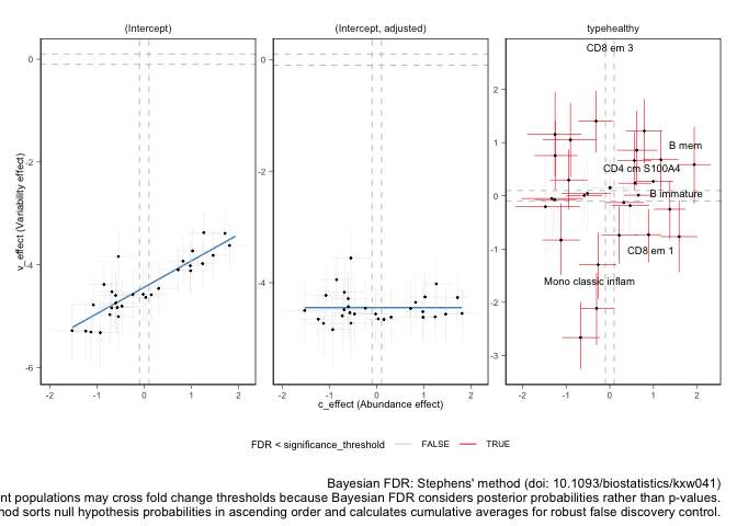
plots$credible_intervals_1DPlot 2D significance plot Data points are cell groups. Error bars are the 95% credible interval. The dashed lines represent the default threshold fold change for which the probabilities (c_pH0, v_pH0) are calculated. pH0 of 0 represent the rejection of the null hypothesis that no effect is observed.
This plot is provided only if differential variability has been tested.
The differential variability estimates are reliable only if the linear
association between mean and variability for (intercept) (left-hand
side facet) is satisfied. A scatterplot (besides the Intercept) is
provided for each category of interest. For each category of interest,
the composition and variability effects should be generally
uncorrelated.
plots$credible_intervals_2DWe recommend setting bimodal_mean_variability_association = TRUE. The
bimodality of the mean-variability association can be confirmed from the
plots$credible_intervals_2D (see below).
We recommend setting bimodal_mean_variability_association = FALSE
(Default).
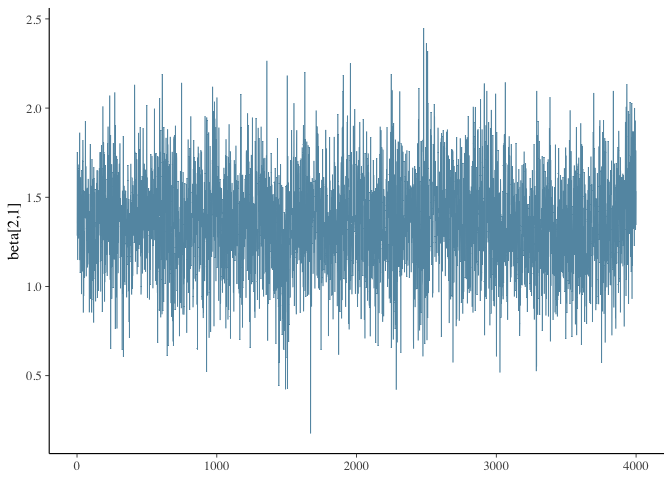
It is possible to directly evaluate the posterior distribution. In this example, we plot the Monte Carlo chain for the slope parameter of the first cell type. We can see that it has converged and is negative with probability 1.
library(cmdstanr)## This is cmdstanr version 0.8.1
## - CmdStanR documentation and vignettes: mc-stan.org/cmdstanr
## - CmdStan path: /Users/a1234450/.cmdstan/cmdstan-2.35.0
## - CmdStan version: 2.35.0
library(posterior)## This is posterior version 1.6.0
##
## Attaching package: 'posterior'
## The following objects are masked from 'package:stats':
##
## mad, sd, var
## The following objects are masked from 'package:base':
##
## %in%, match
library(bayesplot)## This is bayesplot version 1.11.1
## - Online documentation and vignettes at mc-stan.org/bayesplot
## - bayesplot theme set to bayesplot::theme_default()
## * Does _not_ affect other ggplot2 plots
## * See ?bayesplot_theme_set for details on theme setting
##
## Attaching package: 'bayesplot'
## The following object is masked from 'package:posterior':
##
## rhat
# Assuming res contains the fit object from cmdstanr
fit <- res |> attr("fit")

# Extract draws for 'beta[2,1]'
draws <- as_draws_array(fit$draws("beta[2,1]"))

# Create a traceplot for 'beta[2,1]'
mcmc_trace(draws, pars = "beta[2,1]")
The new tidy framework was introduced in 2024, two, understand the differences and improvements. Compared to the old framework, please read this blog post.

