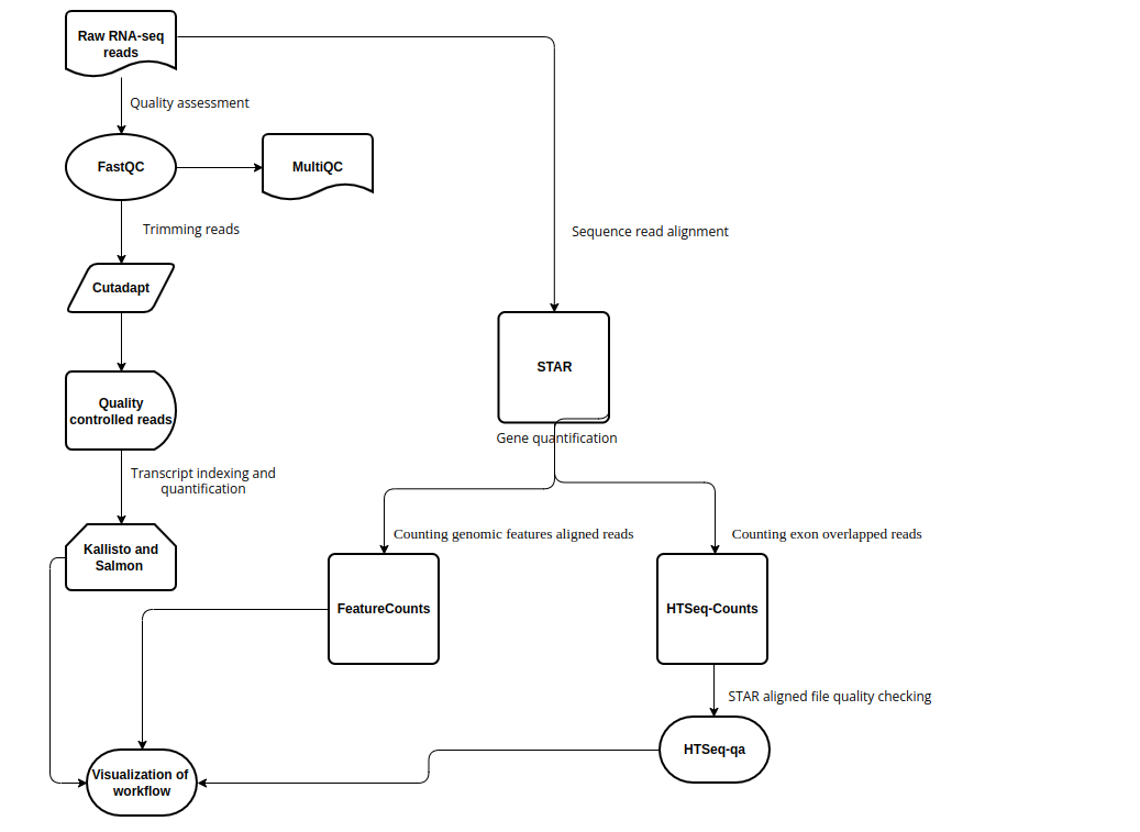
RNA-sequencing (RNA-seq) is a technology to explore the RNA in a sample through high throughput sequencing methods.The extraction of genetic information from RNA-seq data requires a large number of computational tools, with subsequent software and integration of the reference data. Regarding this, RNA-seq data analysis requisites a series of computational steps in a proper sequence, which is performed by a specialized category of workflow management system. Computational steps have been performed to prevent the repetition of steps and making the workflow more precise and effective. Another requirement for the optimized RNA-seq data analysis is that the data analysis should be reproducible and scalable. Snakemake is a useful and worthwhile workflow management system to create reproducible and reliably working data analysis pipelines. The workflow is specified with a customized Snakefile which is based on the Python standard programming language. The file consists of rules about creating output files from input files, workflow dependencies and shell command lines. Here, we have developed an automated workflow in Snakemake to analyze RNA-seq data from different species, using several Bioinformatics tools.
Any Linux based distro should work. Out test OS is:
Distributor ID: Ubuntu
Description: Ubuntu 20.04.3 LTS
Release: 20.04
Codename: focal
lsb_release -a on a Ubuntu based system.
All software should be installed by the user directly as the workflow depends on a lot of external software. Without these the workflow will fail to run.
-
git
-
Jupyter notebook 6.4.11 (python3)
-
PyCharm Professional Edition
-
conda 4.12.0
-
cutadapt 3.4
-
kallisto 0.48.0
-
fastq-dump. 2.8.0
-
FastQC v0.11.9
-
MultiQC 1.12 (ef734c0)
-
fastx-toolkit 0.0.14
-
Salmon 1.8.0
-
Star 2.7.7a
-
Subread v2.0.1
-
htseq-count 2.0.2
-
TUMCS student server
Snakemake (Mölder et al., 2021) is a Python based workflow management tool. In snakemake the entire workflow had distributed into small steps which were defined by specified rules. In regard to execute the command lines in snakemake, “Snakefile” had prepared including inputs (the rules interpret by the dependencies), outputs (the rules interpret by the targets) and the scripts defined in shell blocks. To avoid the repetitions of typing the same pattern fastq file name in Snakemake workflow, "wildcards" (for example: {sample}) had been used. Wildcards returned the sample or multiple samples at a time. Placeholders ({input}, {output}, {threads} and {params}) also implemented in Snakemake workflow. The supplementary parameters correlated to the wildcards were specified by Params. In order to speed up the computation, threads specified in the rules. Snakemake version 7.3.2 had been used here. In snakemake, the dependencies between the rules were determined automatically.
In order to search for the filename matches to the certain filename pattern, and for making the pipeline more generalized and automated, glob wildcard is imported at the beginning of the workflow.
import glob
configfile: "config.yaml"
SAMPLE,=glob_wildcards("{sample}_R1_001.fastq.gz")
To avoid the repetition of typing the same pattern fastq file, {sample} had used as wildcard. One thing to be remembered, the wildcards (here {sample}) can be added to the input, output and params but not in the shell block.
- Sometimes it's necessary to mention the sample root directory (here, SAMPLE_DIR) at the beginning of the workflow to read the sample fastq file. For example, in order for, effective STAR indexing and mapping, featureCounts and HTSeq-count sample directory must be mentioned.
import glob
configfile: "config.yaml"
SAMPLE_DIR="/home/pdebnath/star_snake/"
SAMPLE,=glob_wildcards(SAMPLE_DIR + "/{sample}_R1_001.fastq.gz")
To make the workflow customised, configuration file (configfile) needs to be imported under the glob wildcard. The configuration file should be in JSON or YAML format. The config file we had implemented for the Norway rat (Rattus norvegicus) data analysis represented below:
##config file for Norway rat

adapter_seq: AGATCGGAAGAGC
ref_fasta_sal_kal_rat: http://ftp.ensembl.org/pub/release-104/fasta/rattus_norvegicus/cdna/Rattus_norvegicus.Rnor_6.0.cdna.all.fa.gz
salmon_index_rat: /home/pinky/snakemake_all_rat/salmon_index
SAIndex: 13
ref_star_index_rat: http://ftp.ensembl.org/pub/release-104/fasta/rattus_norvegicus/dna/Rattus_norvegicus.Rnor_6.0.dna.toplevel.fa.gz
ref_gtf_rat: ftp://ftp.ensembl.org/pub/release-89/gtf/rattus_norvegicus/Rattus_norvegicus.Rnor_6.0.89.gtf.gzWe wanted to carry out multiple rules at a time, for that reason we had to mention rule all at the beginning of the Snakefile, which contains all the expected target files as input.
rule all:
    input:
        expand("{sample}_R1_001_fastqc.html",sample=SAMPLE),
        "multiqc_report.html",
        expand("{sample}_R1_001_trimmed.fastq.gz",sample=SAMPLE),
        expand("{sample}_R1_001_trimmed_fastqc.html",sample=SAMPLE),
        expand("kallisto.{sample}/abundance.tsv",sample=SAMPLE),
        expand("salmon.{sample}/quant.sf",sample=SAMPLE)
        expand("{sample}_pass1/SJ.out.tab", sample=SAMPLE),
        expand("{sample}_pass2/Aligned.sortedByCoord.out.bam", sample=SAMPLE),
        expand("{sample}_feature_counts.tsv", sample=SAMPLE),
        expand("{sample}_HTSeq.tsv",sample=SAMPLE)
Here, we wanted to find the FastQC report, MultiQC report, trimmed outcome and FastQC report of the trimmed fastq files, Kallisto and Salmon output, STAR mapping pass-1, STAR mapping pass-2 containing BAM file, FeatureCounts and HTSeq-count output. In a consequence, we had mentioned all the awaited target files as input in rule all. Expand was used to set the wildcard properly and to process all the rules by generating cartesian product.
By providing a .yaml file (env.yaml) in snakemake workflow, Conda environment does need to be created. The env.yaml should mention all of the necessary Bioinformatics toolkits and dependencies.
channels:
    -bioconda
    -conda-forge
    -default
dependencies:
    - cutadapt==3.4
    - kallisto==0.48.0
    - FastQC==v0.11.9
    - MultiQC==1.12 (ef734c0)
    - fastx-toolkit==0.0.14
    - Salmon==1.8.0
    - Star==2.7.7a
    - Subread==v2.0.1
    - htseq-count==2.0.2
- jupyter notebook==6.4.11The Bioinformatics tool FastQC had been used for the quality control check of the sample SRR files. The quality control was based on the per base sequence content and per sequence GC content. For FastQC analysis the following command lines were used in snakemake.
rule fastqc_analysis:
    input:
        R1= "{sample}_R1_001.fastq.gz",
        R2= "{sample}_R2_001.fastq.gz"
    output:
        "{sample}_R1_001_fastqc.html",
        "{sample}_R1_001_fastqc.zip",
        "{sample}_R2_001_fastqc.html",
        "{sample}_R2_001_fastqc.zip"
    shell:
        "fastqc {input.R1} {input.R2}"
Here, the paired-end reads were used, where R1 represent the first read and R2 represent the second read. The snakemake workflow for FastQC analysis in Snakefile defined by the rule fastqc_analysis. FastQC provide the output in HTML and zip file format, that had mentioned in the output section. Instead of fastq file name, wildcard {sample} had implemented to look for all paired end fastq files.
This modular tool had been implemented to accumulate all the bioinformatics result of the provided samples in a single report.
rule run_multiqc:
    input:
        "HSC_T6_S3_R1_001_fastqc.html",
        "HSC_T6_S3_R2_001_fastqc.html"
    output:
        "multiqc_report.html",
        directory("multiqc_data")
    shell:
        "multiqc ."
The obtained fastQC HTML report from FastQC analysis worked here as input and the workflow specified by run_multiqc rule. "multiqc ." implemented in the shell block to get the MultiQC report of all paired-end fastq files.
Cutadapt had implemented for searching and removing the adapters. The adapter removal performed in several steps:
- step-1: Generation of adapters:
rule making_seq_adapter:
    output:
        temp("adapterSeq.fa")
    shell:
        """
        echo -e ">illumina_adapter_forward\n{config[adapter_seq]}" > adapterSeq.fa
"""- Step-2: Computing reverse complement sequence using fastx-toolkit:
Fastx-toolkit is a collection of command line tools implemented for the preprocessing of fastq files. To keep the 5’ and 3’ ends oriented properly reverse complement sequence computed. The adapter sequence and reverse complement sequence downloaded as temporary output, that removed later by Snakemake.
rule compute_reverse_complement:
    input:
        "adapterSeq.fa"
    output:
        temp("adapterSeqRevComp.fa")
    shell:
        "fastx_reverse_complement -i {input} -o {output}"
**** Temporary files: Snakemake can remove the extra output when it is unnecessary. For this motive, we have to spot the temporary output as temp (For example, in our case, temp("adapterSeq.fa") and temp("adapterSeqRevComp.fa") )
--- Here, making_seq_adapter and compute_reverse_complement rules were applied for the generation of sequence adapter and for computing reverse complement sequence.
- Step-3: Adapter removal:
The adapter had been removed by adding Cutadapt in the Conda environment.
rule cutadapt:
    input:
        adapter_reserve_complement = "adapterSeqRevComp.fa",
        R1= "{sample}_R1_001.fastq.gz",
        R2= "{sample}_R2_001.fastq.gz"
    output:
        R1="{sample}_R1_001_trimmed.fastq.gz",
        R2="{sample}_R2_001_trimmed.fastq.gz"
    shell:
        "cutadapt -a {config[adapter_seq]} -A $(tail -n1 {input.adapter_reserve_complement}) -o {output.R1} -p {output.R2} {input.R1} {input.R2}"
To remove adapter in the given paired-end reads, Cutadapt uses -a option for the first read and -A option for the second read. Here, R1 (HSC_T6_S3_R1_001.fastq.gz) is the first read and R2 (HSC_T6_S3_R2_001.fastq.gz) is the second read of our paired-end sample. Reverse complement sequence used as input for trimming. The trimming through Cutadapt was defined by rule cutadapt.
In response to quantification of transcripts, Kallisto and Salmon both are one of the most reliable and faster tools. Rather than direct alignment, the quantification relay on pseudoalignment in both of the tools. For Kallisto and Salmon analysis in our sample Rattus norvegicus (Norway rat), Rattus_norvegicus.Rnor_6.0.cdna.all.fa.gz worked as reference fasta to generate transcriptome index. The reference fasta had downloaded firstly, then extracted as the reference fasta downloaded in zip file format.
rule download_ref:
    input:
    output:
        "Rattus_norvegicus.Rnor_6.0.cdna.all.fa.gz"
    shell:
        "wget -c {config[ref_fasta_sal_kal_rat]}"

rule extract_ref:
    input:
        "Rattus_norvegicus.Rnor_6.0.cdna.all.fa.gz"
    output:
        "Rattus_norvegicus.Rnor_6.0.cdna.all.fa"
    shell:
        "gzip -d {input}"
Regarding Kallisto, quantification occurs in two steps:
- Step-1: Kallisto Indexing:
rule create_index_kallisto:
    input:
        "Rattus_norvegicus.Rnor_6.0.cdna.all.fa"
    output:
        "transcripts.idx"
    shell:
        "kallisto index -i {output} {input}"
Indexing reference fasta marked by create_index_kallisto rule. The reference fasta used as input here. -i indicated index.
- Step-2: Kallisto Quantification:
rule kallisto_quant:
    input:
        index = "transcripts.idx",
        R1   = "{sample}_R1_001_trimmed.fastq.gz",
        R2   = "{sample}_R2_001_trimmed.fastq.gz",

    output:
        "kallisto.{sample}/abundance.tsv"

    shell:
        "kallisto quant -i {input.index} -o kallisto.{wildcards.sample} {input.R1} {input.R2}"
The transcript quantification by kallisto specified by kallisto_quant rule.
Here, -i indicated index and -o output directory. {input} worked as placeholder. The output would be abundance estimated plaintext file (abundance.tsv), which had specified in Output section.
Regarding Salmon quantification occurs in three steps:
- Step-1: Creating salmon indexing directory:
rule salmon_directory:
    output:
        directory("salmon_index")
    shell:
        "mkdir {output} && "
In regard to salmon, the salmon directory had created to store salmon indexed data.
- Step-2: Salmon Indexing:
rule create_index_salmon:
    input:
        "Rattus_norvegicus.Rnor_6.0.cdna.all.fa"
    output:
        directory("{SALMON_INDEX}/transcripts.idx")
    shell:
"salmon index --gencode -p 12 -t {input} -i {output}"- Step-3: Salmon Quantification:
rule salmon_quant:
    output:
        "salmon.{sample}/quant.sf",
    input:
        index = "salmon_index/transcripts.idx",
        R1   = "{sample}_R1_001_trimmed.fastq.gz",
        R2   = "{sample}_R2_001_trimmed.fastq.gz",

    shell:
        "salmon quant -i {input.index} -l A -p 12 --gcBias "
        "--numGibbsSamples 20 --thinningFactor 100 "
        "-o salmon.{wildcards.sample} -1 {input.R1} -2 {input.R2}"
Unlike Kallisto, initially, in Salmon, the salmon directory had to be created, to store indexed data. Afterward, the quantification of transcripts performed. The salmon_directory, create_index_salmon, salmon_quant rules had implemented to create the salmon directory, salmon indexing and salmon transcripts quantification. In Salmon, the estimation of the variance in estimated transcripts abundance (--numGibbsSamples) and the correction of GC biases (--gcBias) had carried out with 12 threads (-p 12) for quasi-mapping.
Salmon output is a plain-text, tab-seperated file (quant.sf) including name, length, effective length, Transcript per million (TPM) value and number of reads of the target transcript.
- To access the wildcard values through attribute, {wildcards.sample} implemented.
STAR referred to as Spliced Transcripts Alignment to a Reference, is a read mapper for RNA sequencing data. STAR mapping occurred in two steps, including star indexing and star read mapping.
- Step-1:STAR Indexing:
The first step of the STAR alignment was the indexing of the reference genome. For indexing, the implemented reference genome sequence was Rattus_norvegicus.Rnor_6.0.dna.toplevel.fa for Rattus norvegicus. Moreover, as reference annotation Rattus_norvegicus.Rnor_6.0.89.gtf had applied.
rule star_indexing:
	input:
		fasta="Rattus_norvegicus.Rnor_6.0.dna.toplevel.fa",
		gtf="Rattus_norvegicus.Rnor_6.0.89.gtf"
	output:
		directory("starIndex")
	threads: 20
	shell:
		'mkdir {output} && '
		'STAR --runThreadN {threads} '
		'--runMode genomeGenerate '
		'--genomeDir {output} '
		'--genomeFastaFiles {input.fasta} '
		'--sjdbGTFfile {input.gtf} '
		'--sjdbOverhang 100'
Indexing of STAR specified by star_indexing rule.
Here,
-
--genomeDir indicates the root of the directory, where the genome indices to be stored.
-
--runMode genomeGenerate is a direction toward genome indices generation.
-
--runThreadN {threads} specifies the number of threads for the genome generation.
-
--genomeFastaFiles {input.fasta} indicates the specified input reference fasta file.
-
--sjdbOverhang is used to concatenate bases from the junctions of donor and acceptor sides.
-
--sjdbGTFfile represent the input GTF file path with annotations.
-
{input}, {output} and {params} work as placeholder.
-
The output include starIndex directory, to store the indexed star data.
-
The output directory is created by mkdir.
- Step-2:Star read mapping:
The second step was mapping the reads. Here, 2-pass mapping had done. The 1st pass was getting alignment and splice junction information, then 2nd pass of the mapping was done by using the splice junction information, that was generated from the 1st pass of mapping and the read counting was performing at the same time.
rule star_pass1:
	input:
		R1=SAMPLE_DIR+"HSC_T6_S3_R1_001.fastq.gz",
		R2=SAMPLE_DIR+"HSC_T6_S3_R2_001.fastq.gz",
		ref_dir=SAMPLE_DIR+"starIndex"

	params:
		outdir="{sample}_pass1"

	output:
		"{sample}_pass1/SJ.out.tab"
	threads: 20
	shell:
		'rm -rf {params.outdir} &&'
		'mkdir {params.outdir} && '
		'cd {params.outdir} && '
		'STAR --runThreadN {threads} '
		'--genomeDir {input.ref_dir} '
		'--readFilesIn {input.R1},{input.R2} '
		'--readFilesCommand zcat '
		'--outSAMtype BAM Unsorted '

rule star_pass2:
	input:
		R1=SAMPLE_DIR+"HSC_T6_S3_R1_001.fastq.gz",
		R2=SAMPLE_DIR+"HSC_T6_S3_R2_001.fastq.gz",
		ref_dir=SAMPLE_DIR+"starIndex",
		sj=SAMPLE_DIR+"{sample}_pass1/SJ.out.tab"
	params:
		outdir="{sample}_pass2",
		id="{sample}"
	output:
		"{sample}_pass2/Aligned.sortedByCoord.out.bam"
	threads: 20
	shell:
		'rm -rf {params.outdir} &&'
                'mkdir {params.outdir} && '
                'cd {params.outdir} && '
                'STAR --runThreadN {threads} '
                '--genomeDir {input.ref_dir} '
                '--readFilesIn {input.R1},{input.R2} '
                '--readFilesCommand zcat '
                '--outSAMtype BAM SortedByCoordinate '
	        '--outSAMattrRGline ID:{params.id} '
                '--sjdbFileChrStartEnd {input.sj} '
                '--quantMode GeneCounts '
Here,
- rule star_pass1 and rule star_pass2 specifies the 2-pass mapping.
- Params defined the output directory where the pass-1 and pass-2 mapping results have been stored.
- Placeholders define the {input} {output} and {params}.
- The number of reads per gene counted here by --quantMode GeneCounts.
** The output of the STAR mapping is the binary aligned file (BAM file).
In order to count the number of reads align to the genomic features, featuresCounts had used. The input BAM file was Aligned.sortedByCoord.out.bam generated from the STAR mapping and the sample GTF file was Rattus_norvegicus.Rnor_6.0.89.gtf for Norway Rat (Rattus norvegicus).
rule feature_count:
    input:
        bam = SAMPLE_DIR+"{sample}_pass2/Aligned.sortedByCoord.out.bam",
        gtf= SAMPLE_DIR+"Rattus_norvegicus.Rnor_6.0.89.gtf"
    output:
        "{sample}_feature_counts.tsv"
    threads: 20
    shell:
        "featureCounts -T 4 -t exon -g gene_id -a {input.gtf} -o {output} {input.bam}"
Here,
- The featureCounts workflow had specified in rule feature_count.
- The input file location directory had mentioned in SAMPLE_DIR (SAMPLE_DIR="/home/pdebnath/star_snake/").
- Aligned.sortedByCoord.out.bam (STAR aligned BAM file) used to count the reads through aligning the sample GTF file.
To find the number of reads overlapping it’s exons, htseq-count executed.
rule htseq:
    input:
        bam = SAMPLE_DIR+"{sample}_pass2/Aligned.sortedByCoord.out.bam",
        gtf= SAMPLE_DIR+"Rattus_norvegicus.Rnor_6.0.89.gtf"
    output:
        "{sample}_HTSeq.tsv"
    threads: 2
    shell:
        "samtools view -h {input.bam} | htseq-count --mode intersection-strict --stranded no --minaqual 1 --type exon --idattr gene_id - {input.gtf} > {output}"
Here,
- The htseq-count snakemake workflow defined by rule htseq.
- The input file had specified by BAM ( Aligned.sortedByCoord.out.bam) and annotated GTF file ( Rattus_norvegicus.Rnor_6.0.89.gtf) with specified root directory.
- The wildcard {sample} had used ((HSC_T6_S3)- rat genome)).
- Samtools view used to convert the aligned BAM file (binary file) into the SAM file (text based).
- For HTSeq-count, gene ID and exon had attributed.
** In order to speed up the computation of HTSeq-count, Snakemake do need threads more than 1 and need to be specified.
The generated STAR aligned BAM file quality can be checked through python based htseq-qa. Htseq-qa carried out in two steps.
- Step-1:
For htseq-qa the first step was to convert the aligned BAM file to SAM (defined by rule converting_bam_to_sam_file in Snakemake workflow).
rule converting_bam_to_sam_file:
    input:
        "Aligned.sortedByCoord.out.bam"
    output:
        "Aligned.sortedByCoord.out.sam"
    shell:
"samtools view -h {input} > {output} "- Step-2:
The next step was to perform quality assessment of the BAM file (describe by rule htseq_qa in Snakemake workflow).
rule htseq_qa:
    input:
        "Aligned.sortedByCoord.out.sam"
    output:
        "Aligned.sortedByCoord.out.sam.pdf"

    shell:
        "python -m HTSeq.scripts.qa {input} "
For each rule, input file, output file and command lines were specified in shell block in Snakefile.
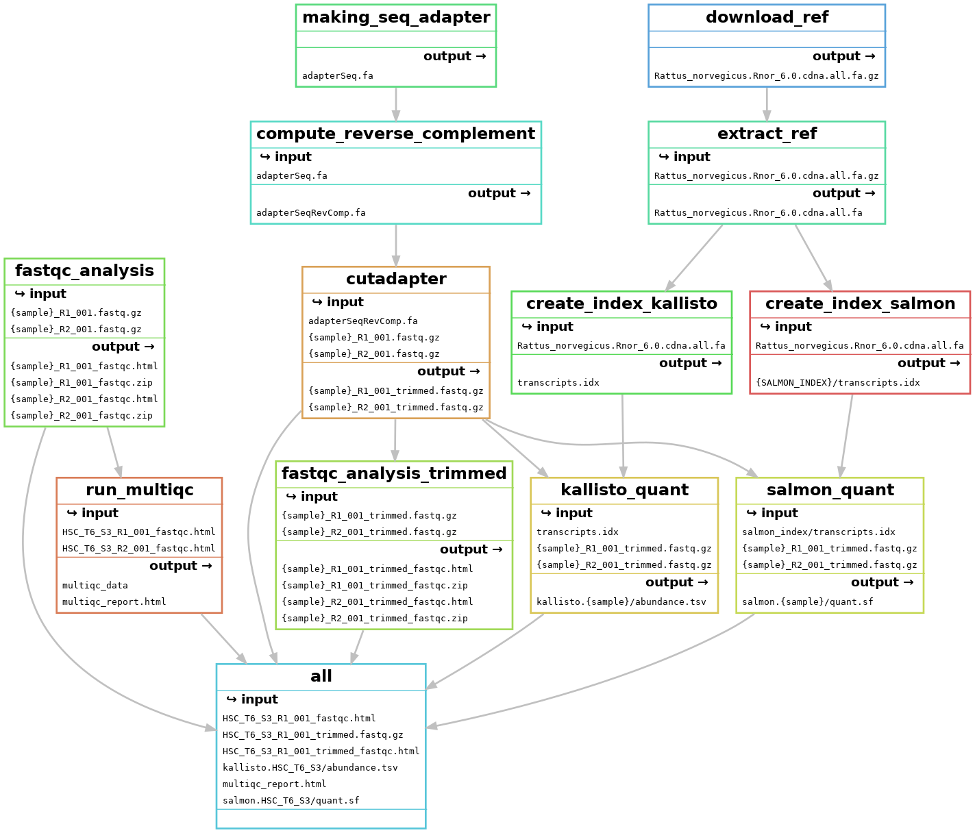
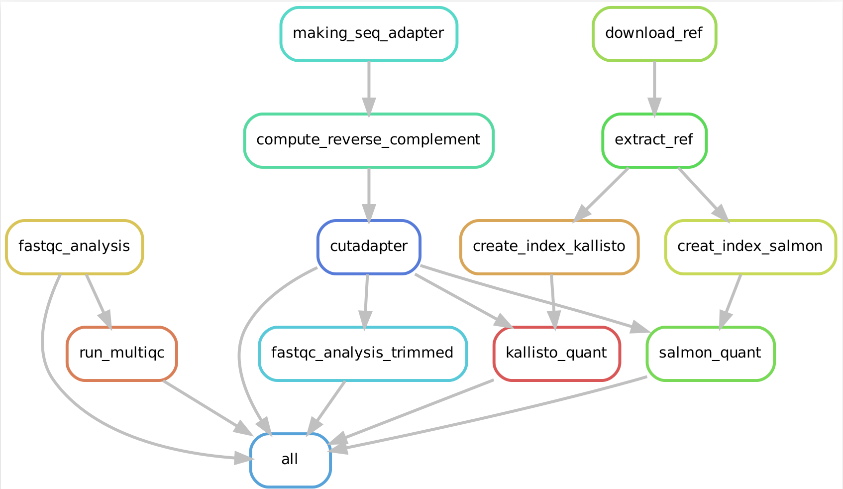
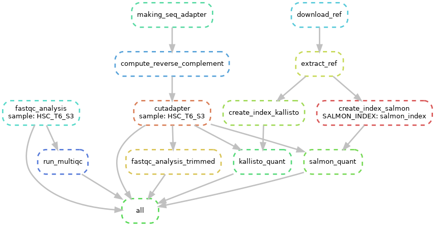
Snakemake workflow can be represented in filegraph, rulegraph and DAG (direct acrylic graph). Filegraph mentions each and every detail, including all input and output files. Rulegraph displays only the correlation between the rules. DAG graph presents the dependencies and the rules for each job. The path represents the sequence of jobs executed consecutively. The nodes constitute for execution of rules. The Snakemake workflow visualization can be performed in the following ways:
- Visualization as filegraph
snakemake --filegraph | dot -Tpng > filegraph.png- Visualization as rulegraph
snakemake --rulegraph | dot -Tpng > rulegraph.png- Visualization as Direct Acrylic Graph (DAG)
snakemake --dag | dot -Tpng > dag.png-
The overall workflow from FastQC analysis to the Salmon and Kallisto analysis is represented visually in filegraph, rulegraph and dag (direct acrylic graph):
Snakemake cen generate report consists of runtime statistics, workflow topology and results as HTML.
snakemake --report snakemake_workflow_report.htmlTranscript per million (TPM) is a normalization method for RNA-seq data.Transcripts Per Million ratio can be counted in following ways (Li et al., 2010) (Pachter, 2011) :
-
Counting RPK (Reads per Kilobase): Each gene read counts have to be divided by each gene length.
RPK=Read Counts/ (gene length * 0.001) -
Generating per million scaling factor and counting TPM: Sum up all the RPK values and dividing the number by 1000,000. And then divide the RPK values with per million scaling factor and TPM will be counted.
           Per million scaling factor= ΣRPK/10^6

      TPM= Each gene RPK values/per million scaling factor
Therefore, Snakemake workflow is automated and reproducible enough for the analysis and re-analysis of the paired-end RNA-seq dataset. It is expected that the advances in automating the generated workflow will facilitate to study the distinct type of RNA-seq data.
- Mölder, F., Jablonski, K. P., Letcher, B., Hall, M. B., Tomkins-Tinch, C. H., Sochat, V., ... & Köster, J. (2021). Sustainable data analysis with Snakemake. F1000Research, 10.
- Pachter, L. (2011). Models for transcript quantification from RNA-Seq. arXiv preprint arXiv:1104.3889.
- Li, B., Ruotti, V., Stewart, R. M., Thomson, J. A., & Dewey, C. N. (2010). RNA-Seq gene expression estimation with read mapping uncertainty. Bioinformatics, 26(4), 493-500.


