Single-Shot Cuboids: Geodesics-based End-to-end Manhattan Aligned Layout Estimation from Spherical Panoramas

This repository contains the code and models for the paper "Single-Shot Cuboids: Geodesics-based End-to-end Manhattan Aligned Layout Estimation from Spherical Panoramas".

Parts of the code can be used for keypoint localisation using spherical panorama inputs (projected in the equirectangular domain).

Usage

Inference

To use the pretrained model and receive its predictions on panorama images run:

                        python inference.py 'GLOB_PATH'

where GLOB_PATH can be a single filename (image.jpg), or a folder search pattern (path/to/images/*.jpg).

Additional options are:

--model MODEL: Use a different model, available choices include:
- ssc: The real-world data trained Single-Shot Cuboids model. (this is the default mode)
- ssc_syn: The synthetic data trained Single-Shot Cuboids model.
- hnet: The real-world data trained HorizonNet model.
- hnet_syn: The synthetic data trained HorizonNet model.
--output_path PATH_TO_SAVE_RESULTS: An existing folder where the predictions will be saved at. (default: '.')
--gpu INTEGER_ID: Select a different GPU to run inference on.(default: 0)
--floor_distance NEGATIVE_FLOAT_VALUE: Used when saving the resulting meshes and during cuboid fitting. (default: -1.6m)
--remove_ceiling: Using this flag will remove the ceiling from the resulting meshes.
--save_boundary: Using this flag will save a visualization of the layout wireframe on the panorama.
--save_mesh: Using this flag will save a textured mesh of the result.
--mesh_type: A choice for the mesh output. Can be either obj or usdz for Wavefront and Pixar's formats respectively.

Serve

It is also possible to use the models via torchserve.

The scripts/torchserve_create_*.bat shell scripts create the .mar files found in /mars (pre-archived ones are also available).

These can be used to serve these models using REST calls by executing the scripts/torchserve_run_*.bat shell scripts. Upon serving them the endpoints are reachable at http://IP:8080/predictions/MODEL_NAME, with IP as selected when configuring torchserve (typically localhost, but more advanced configuration is also possible to serve models externally or make them reachable from other machines, using the inference_address setting). The MODEL_NAME is the same as the --model MODEL_NAME flag mentioned above.

A callback URL based json payload needs to be POSTed to retrieve predictions:

"inputs": {
  "color": "GET_IMAGE_URL"
},
"outputs": {
  "boundary": "POST_BOUNDARY_URL",
  "mesh": "POST_MESH_URL"
},
"floor_distance": NEGATIVE_FLOAT_VALUE,
"remove_ceiling": BOOLEAN_VALUE,

Apart from the latter two options which are optional and take the default values mentioned above, the GET/POST callback URLs are serving inference images (GET), or saving predicted results (POST).

An image and results server is provided and started via:

                        python panorama_server.py 'GLOB_PATH'

which hosts all images given in GLOB_PATH at http://IP:PORT/FILENAME. It also offers an exporting endpoint at http://IP:PORT/save/FILENAME which saves the corresponding output files.

Other arguments apart from the input panorama glob path are:

--output_path PATH_TO_SAVE_RESULTS: An existing folder where the predictions will be saved at. (default: '.')
--ip ADDRESS_STRING: The IP address where the endpoint will be reachable at. (default: localhost)
--port PORT_NUMBER: The port number where the endpoint will be reachable at. (default: 5000)

Once the models are served and the panorama server is running, at the INFERENCE_SERVER_ENDPOINT and IMAGE_SERVER_ENDPOINT respectively, a prediction is callable via:

curl -H "Content-Type: application/json" -d "{\"inputs\": {\"color\":
\"http://IMAGE_SERVER_ENDPOINT/image.jpg\"}, \"outputs\": {\"boundary\": \"http://IMAGE_SERVER_ENDPOINT/save/boundary_image.jpg\", \"mesh\":
\"http://IMAGE_SERVER_ENDPOINT/save/mesh.obj\"}}"
http://INFERENCE_SERVER_ENDPOINT/predictions/ssc

The outputs arguments are optional and can be omitted if no result saving is required. The response will include in json format a list of lists denoting the layout corner pixel positions in interleaving top/bottom/top/bottom/etc. order.

Assuming that the model and panorama server are hosted locally with their default ports and the input image is img.png then the REST command for the ssc model is:

curl -H "Content-Type: application/json" -d "{\"inputs\": {\"color\":
\"http://localhost:5000/img.png\"}, \"outputs\": {\"boundary\":
\"http://localhost:5000/save/img.jpg\", \"mesh\":
\"http://localhost:5000/save/img.obj\"}}"
http://localhost:8080/predictions/ssc

Download

The ./ckpt and ./mar folders should contain the torch checkpoint saved files for all models, as well as the torch archives for serving them. To download them either run the download.bat scripts at the respective folders, or check the README instructions to download them manually from the respective releases.

Modules

Plug-n-play modules of the different components are also available and ready to be integrated.

Geodesic Distace

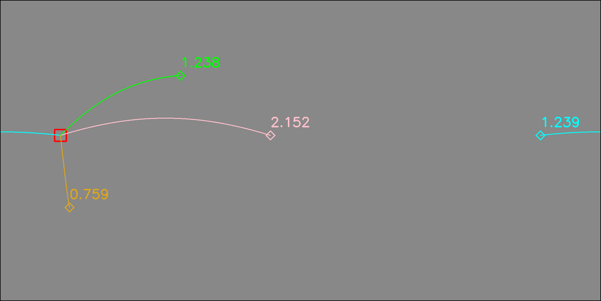
The GeodesicDistance module found in ./ssc/geodesic_distance.py calculates the great circle or harvesine distance of two coordinates on the sphere. The following image shows the harvesine distance and the corresponding great circle path between points on the equirectangular domain. Distances from the red square to the colored diamonds are also reported in the corresponding color.

                            loss = GeodesicDistance()

An interactive comparison between the geodesic distance and the L2 distance can be run with:

                        python ssc/geodesic_distance.py

Left clicking selects the first (left hand side) point, and right clicking the corresponding second (right hand side) point. Upon having selected a left and right point, their geodesic and L2 distance will be printed.

Geodesic Heatmaps

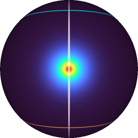
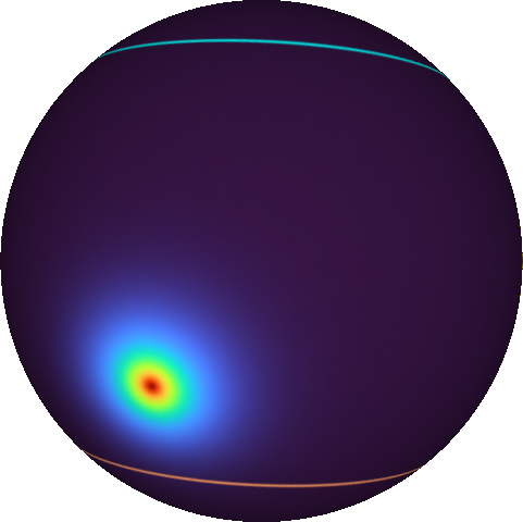
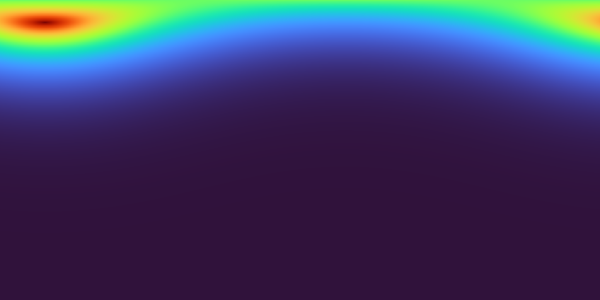
The GeodesicGaussian module found in ./ssc/geodesic_gaussian.py relies on the geodesic distance and reconstructs a Gaussian distribution directly on the equirectangular domain that respects the continuity around the horizontal boundary, and, at the same time, is aware of the equirectangular projection's distortion.

                  module = GeodesicGaussian(std=9.0, normalize=True)

The following images show a Gaussian distribution defined on the sphere (left) and the corresponding distribution reconstructed on the equirectangular domain (right).

Different (20) random centroid distributions can be visualized by runningwith:

                python ssc/geodesic_gaussian.py {std: float=9.0} {width: int=512}

with the (optional) std argument given in degrees (default: 9.0), and the (optional) width argument defining the equirectangular pixels at the longitudinal angular coordinate (default: 512).

Quasi-Manhattan Center of Mass

The QuasiManhattanCenterOfMass module found in ./ssc/quasi_manhattan_center_of_mass.py estimates the meridian-aligned top and bottom corners using either:

the standard mode that calculates the default center of mass (CoM), or,
the periodic mode which calculates a boundary aware spherical center of mass.

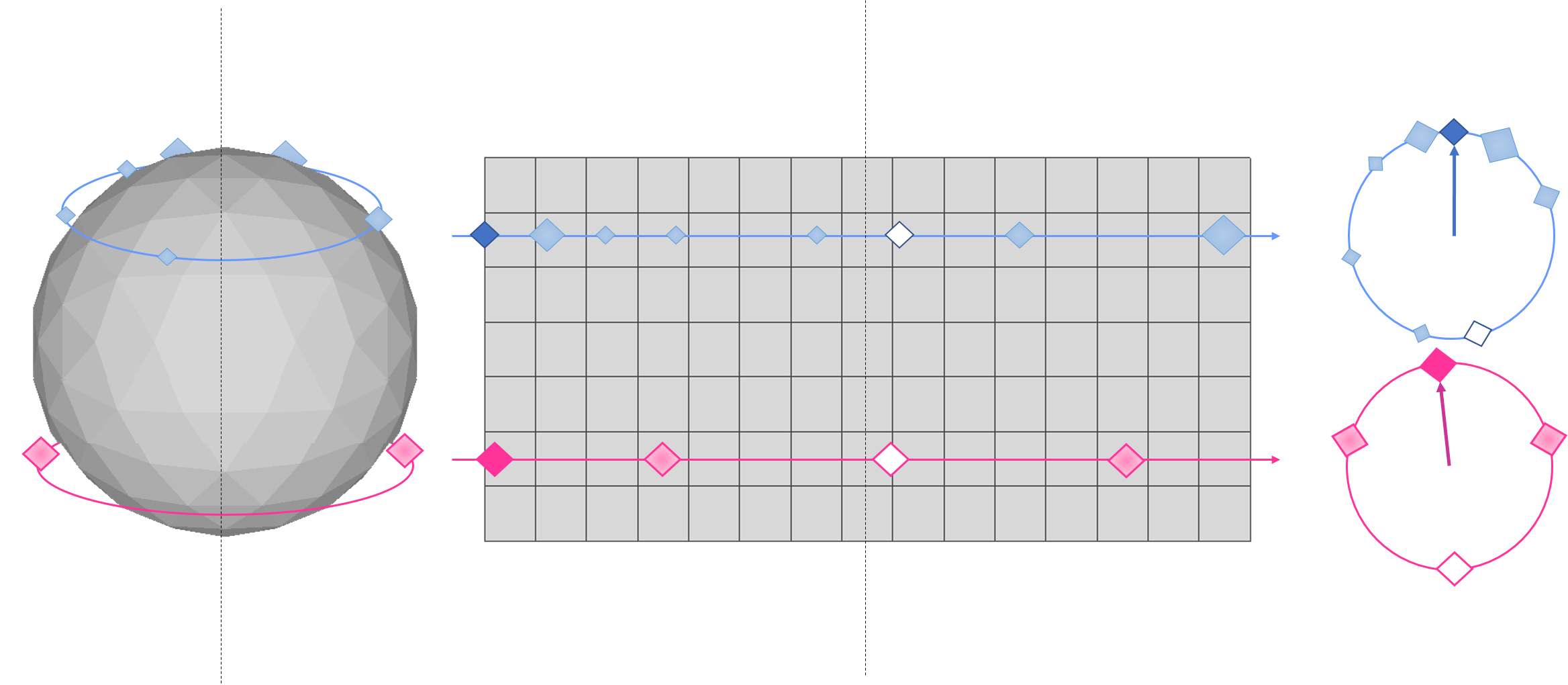
                module = QuasiManhattanCenterOfMass(mode='periodic')

Their differences are depicted in the following figure, where the CoM of a set of blue or pink particles, whoses masses are denoted by their size, is estimated with both methods on an equirectangular grid. The standard method (white filled particles) fails to properly localize the CoM as it neglects the image's continuity around the horizontal boundary. The periodic method (darker filled colored particles) resolves this issue taking into account the continuous boundary.

The input to the module's forward function is:

a [W x H] grid G with coordinates normalized to [-1, 1], and,
the predicted heatmap H.

                       corners = scom.forward(grid, gaussian)

An example with randomly allocated points, their geodesic gaussian reconstruction and the corresponding localisations using a normalized grid can be seen by running:

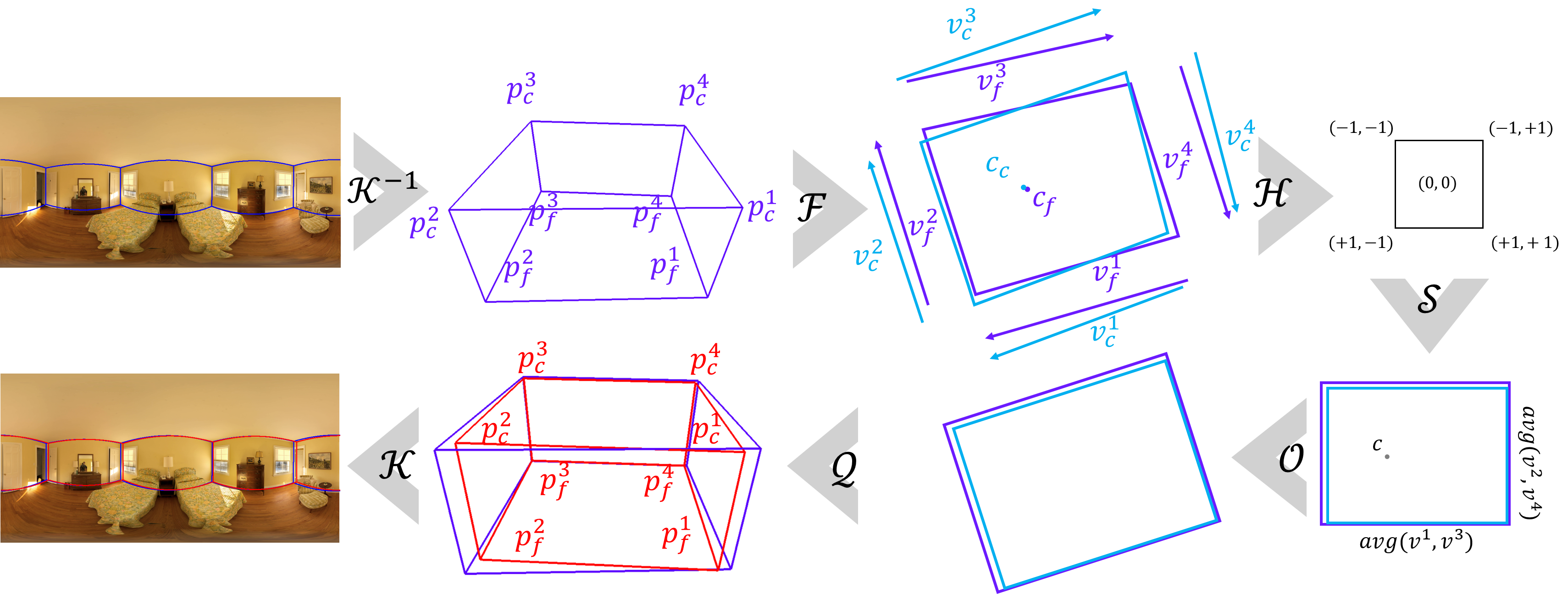
    python ssc/quasi_manhattan_center_of_mass.py '{mode: standard|periodic}'

Cuboid Fitting

The CuboidFitting module found in ./ssc/cuboid_fitting.py fits a cuboid into 8 estimated corner locations as described in the paper and depicted in the following figure.

                      head = CuboidFitting(mode='joint')

A set of examples can be run using:

      python ssc/cuboid_fitting.py '{test: [1-7]]} {mode: floor|ceil|avg|joint}'

where one of 7 test cases can be selected and one of the available modes:

floor for using the floor as a fixed height plane,
ceil for using the ceiling as a fixed height plane,
avg for using both and averaging their projected coordinates, and,
joint for fusing the floor view projected floor and ceiling coordinates.

The original coordinates will be colored blue, while the cuboid fitted coordinates will be colored green.

Examples on the different test sets follow, with the images on the left being the predicted coordinates floor plan view, and the images on the right those after cuboid fitting:

Sun360

Stanford2D3D

Structured3D

Kujiale

Spherically Padded Convolution

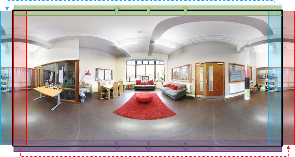
The SphericalConv2d module in ./ssc/spherically_padded_conv.py applies the padding depicted below that adapts traditional convs to the equirectangular domain by replication padding at the singularities/poles and circular padding around the horizontal boundary.

Citation

If you used or found this code and/or models useful, please cite the following:

@article{zioulis2021singleshot,
title = {Single-shot cuboids: Geodesics-based end-to-end Manhattan aligned layout estimation from spherical panoramas},
author = {Nikolaos Zioulis and Federico Alvarez and Dimitrios Zarpalas and Petros Daras},
journal = {Image and Vision Computing},
volume = {110},
pages = {104160},
year = {2021},
issn = {0262-8856},
doi = {https://doi.org/10.1016/j.imavis.2021.104160},
url = {https://github.com/VCL3D/SingleShotCuboids},
keywords = {Panoramic scene understanding, Indoor 3D reconstruction, Layout estimation, Spherical panoramas, Omnidirectional vision}
}

Acknowledgements

This project has received funding from the European Union’s Horizon 2020 research and innovation programme ATLANTIS under grant agreement No 951900.

Parts of the code used in this work have been borrowed or adapted from these repositories:

Structured3D from Jia Zheng
Anti-aliased CNNs from Richard Zhang
HorizonNet from Cheng Sun
Stacked Hourglass from Chris Rockwell
Svd Gist from Muhammed Kocabas
The panorama_server.py is based on a template image server created by Werner Bailer