Although recent efforts have shown that structural variations (SVs) can disrupt the 3D genome organization and induce enhancer-hijacking, no computational tools exist to detect such events from chromatin interaction data, such as Hi-C. Here, we develop NeoLoopFinder, a computational framework to identify the chromatin interactions induced by SVs, such as inter-chromosomal translocations, large deletions, and inversions. Our framework can automatically reconstruct local Hi-C maps surrounding the breakpoints, normalize copy number variation and allele effects, and capture local optimal signals. We applied NeoLoopFinder in Hi-C data from 50 cancer cell lines and primary tumors and identified tens of recurrent genes associated with enhancer-hijacking in different cancer types. To validate the algorithm, we deleted hijacked enhancers by CRISPR/Cas9 and showed that the deletions resulted in the reduction of the target oncogene expression. In summary, NeoLoopFinder is a novel tool for identifying potential tumorigenic mechanisms and suggesting new diagnostic and therapeutic targets.
Wang, X., Xu, J., Zhang, B., Hou, Y., Song, F., Lyu, H., Yue, F. Genome-wide detection of enhancer-hijacking events from chromatin interaction data in re-arranged genomes. Nat Methods. 2021.
NeoLoopFinder and all the dependencies can be installed using either mamba or pip:
$ conda config --add channels r
$ conda config --add channels defaults
$ conda config --add channels bioconda
$ conda config --add channels conda-forge
$ conda config --set channel_priority strict
$ mamba create -n neoloop cooler matplotlib pyensembl pybigwig intervaltree rpy2 r-mgcv scikit-learn=1.1.2 joblib=1.1.0 "pomegranate<=0.14.8"
$ mamba activate neoloop
$ pip install -U neoloop TADLib
neoloop-finder is distributed with 9 scripts. You can learn the basic usage of each script
by typing command [-h] in a terminal window, where "command" is one of the following
script names:
calculate-cnv
Calculate the copy number variation profile from Hi-C map using a generalized additive model with the Poisson link function
segment-cnv
Perform HMM segmentation on a pre-calculated copy number variation profile.
plot-cnv
Plot genome-wide CNV profiles and segments.
correct-cnv
Remove copy number variation effects from cancer Hi-C.
simulate-cnv
Simulate CNV effects on a normal Hi-C. The inputs are the Hi-C matrix of a normal cell in .cool format, the Hi-C matrix of a cancer cell in .cool format, and the CNV segmentation file of the same cancer cell in bedGraph format.
assemble-complexSVs
Assemble complex SVs. The inputs are a list of simple SVs and the Hi-C matrix of the same sample.
neoloop-caller
Identify neo-loops across SV breakpoints. The required inputs are the output SV assemblies from
assemble-complexSVsand the corresponding Hi-C map in .cool format.neotad-caller
Identify neo-TADs. The inputs are the same as
neoloop-caller.searchSVbyGene
Search SV assemblies by gene name.
This tutorial will cover the overall pipeline of NeoLoopFinder. Given a Hi-C map in .cool/.mcool format and an SV list in the same sample, NeoLoopFinder starts with the inference of the genome-wide copy number variation (CNV) profile and remove the CNV effects from Hi-C. Then it resolves complex SVs and reconstructs local Hi-C matrices surrounding SV breakpoints. And finally, it detects chromatin loops on each SV/complex SV assembly, including both loops in the regions not affected by SVs and loops across the breakpoints.
Note
If the chromosome names in your .cool files do not have the "chr" prefix,
please make sure to add the "chr" prefix using add_prefix_to_cool.py
before you run calculate-cnv (issue #1).
Also make sure you have run cooler balance on your cool files before
you run correct-cnv (issue #8).
First, let's download a processed Hi-C dataset in SK-N-MC (a neuroepithelioma cell line):
$ wget -O SKNMC-MboI-allReps-filtered.mcool -L https://www.dropbox.com/s/tuhhrecipkp1u8k/SKNMC-MboI-allReps-filtered.mcool?dl=0
The downloaded ".mcool" file contains contact matrices at multiple resolutions. To list all
individual cool URIs within it, execute the cooler ls command below:
$ cooler ls SKNMC-MboI-allReps-filtered.mcool

SKNMC-MboI-allReps-filtered.mcool::/resolutions/5000
SKNMC-MboI-allReps-filtered.mcool::/resolutions/10000
SKNMC-MboI-allReps-filtered.mcool::/resolutions/25000
SKNMC-MboI-allReps-filtered.mcool::/resolutions/50000
SKNMC-MboI-allReps-filtered.mcool::/resolutions/100000
SKNMC-MboI-allReps-filtered.mcool::/resolutions/250000
SKNMC-MboI-allReps-filtered.mcool::/resolutions/500000
SKNMC-MboI-allReps-filtered.mcool::/resolutions/1000000
SKNMC-MboI-allReps-filtered.mcool::/resolutions/2500000
SKNMC-MboI-allReps-filtered.mcool::/resolutions/5000000
To infer the genome-wide CNV profile at a specific resolution, just run calculate-cnv using the cool URI at that resolution as input. For example, the following command will calculate the CNV profile at the 25kb resolution:
$ calculate-cnv -H SKNMC-MboI-allReps-filtered.mcool::resolutions/25000 -g hg38 \
                -e MboI --output SKNMC_25k.CNV-profile.bedGraph
Here the -g parameter indicates the reference genome you used for mapping
your Hi-C data, which currently supports hg38, hg19, mm10, and mm9.
And the "-e" parameter indicates the restriction enzyme used in your
Hi-C experiment, which currently supports HindIII, MboI, DpnII, BglII,
Arima, and uniform, where uniform may be specified when the genome was
cutted using a sequence-independent/uniform-cutting enzyme
(please refer to issue 24).
The inferred CNV values for each 25kb bin will be reported in the bedGraph format as follows:
$ head SKNMC_25k.CNV-profile.bedGraph

chr1        0       25000   0.3622223616602325
chr1        25000   50000   0.16018489189648388
chr1        50000   75000   0.6700770894724766
chr1        75000   100000  0.29407421138399936
chr1        100000  125000  0.7064836696780397
chr1        125000  150000  0.18356628377821504
chr1        150000  175000  0.008115191530591481
chr1        175000  200000  1.9345786937265874
chr1        200000  225000  1.1066640487666337
chr1        225000  250000  0.0
Since the raw CNV profiles are usually relatively noisy, the next step is to identify CNV segments from the original signals:
$ segment-cnv --cnv-file SKNMC_25k.CNV-profile.bedGraph --binsize 25000 \
              --ploidy 2 --output SKNMC_25k.CNV-seg.bedGraph --nproc 4
Here the --ploidy parameter indicates the ploidy or on average how many chromosome
copies are there in your sample's cell nucleus. For example, in our analysis,
we set this parameter to 2 for diploid/pseudodiploid cells, 3 for triploid/hypotriploid
cells, 4 for hypotetraploid cells, and 5 for hypopentaploid cells. This information
is usually obtained from karyotyping, but if you are not sure about it for your samples,
you can safely set it to 2.
So how does the inferred CNV look like? For this job, you can use the plot-cnv command:
$ plot-cnv --cnv-profile SKNMC_25k.CNV-profile.bedGraph \
           --cnv-segment SKNMC_25k.CNV-seg.bedGraph \
           --output-figure-name SKNMC_25k.CNV.genome-wide.png \
           --dot-size 0.5 --dot-alpha 0.2 --line-width 1 --boundary-width 0.5 \
           --label-size 7 --tick-label-size 6 --clean-mode
If you want to zoom into specific chromosomes, you can specify the chromosome labels
on the command using the -C parameter:
$ plot-cnv --cnv-profile SKNMC_25k.CNV-profile.bedGraph \
           --cnv-segment SKNMC_25k.CNV-seg.bedGraph \
           --output-figure-name SKNMC_25k.CNV.bychrom.png \
           --dot-size 1.5 --dot-alpha 0.3 --line-width 1.5 --boundary-width 1 \
           --label-size 7 --tick-label-size 6 --maximum-value 3 \
           --minimum-value -5 -C 3 4 5 6 7 8
Note that most key parameters of the CNV segmentation algorithm is now tunable since v0.4.1, so if you are not satisfied with the segmentation outputted by the default parameters, it would always be a good idea to tune those parameters yourself to find the best solution (see an example here issue #3).
At the end of this section, let's compute the CNV profiles and CNV segments at 10kb and 5kb resolutions as well:
$ calculate-cnv -H SKNMC-MboI-allReps-filtered.mcool::resolutions/10000 -g hg38 \
                -e MboI --output SKNMC_10k.CNV-profile.bedGraph
$ segment-cnv --cnv-file SKNMC_10k.CNV-profile.bedGraph --binsize 10000 \
              --ploidy 2 --output SKNMC_10k.CNV-seg.bedGraph --nproc 4
$ calculate-cnv -H SKNMC-MboI-allReps-filtered.mcool::resolutions/5000 -g hg38 \
                -e MboI --output SKNMC_5k.CNV-profile.bedGraph
$ segment-cnv --cnv-file SKNMC_5k.CNV-profile.bedGraph --binsize 5000 \
              --ploidy 2 --output SKNMC_5k.CNV-seg.bedGraph --nproc 4
As copy number variations (CNVs) can greatly distort Hi-C signals in cancer cells, we suggest using the correct-cnv command to remove such effects along with other systematic biases including mappability, GC content, and restriction fragment sizes from the Hi-C data.
The command below will perform this CNV normalization on the above SK-N-MC Hi-C at the 25kb resolution:
$ correct-cnv -H SKNMC-MboI-allReps-filtered.mcool::resolutions/25000 \
              --cnv-file SKNMC_25k.CNV-seg.bedGraph --nproc 4 -f
correct-cnv takes the Cool URI at a certain resolution and the CNV segmentation file at the same resolution as inputs, and after this command has been executed, a bias vector will be reported in the "sweight" column in the bins table of the cool file, which can be further used to normalize the Hi-C contacts.
Again, let's perform the CNV normalization at the 10kb and 5kb resolutions as well:
$ correct-cnv -H SKNMC-MboI-allReps-filtered.mcool::resolutions/10000 \
              --cnv-file SKNMC_10k.CNV-seg.bedGraph --nproc 4 -f
$ correct-cnv -H SKNMC-MboI-allReps-filtered.mcool::resolutions/5000 \
              --cnv-file SKNMC_5k.CNV-seg.bedGraph --nproc 4 -f
Note
By default, assemble-complexSVs, neoloop-caller, and neotad-caller
will use the "sweight" column to normalize the Hi-C matrix. However, you can
change this option to ICE normalization by specifying --balance-type ICE.
After you have obtained the CNV-normalized Hi-C matrices, the next step of NeoLoopFinder is to reconstruct the Hi-C map for the rearranged genomic regions surrounding SV breakpoints. This job can be done by the assemble-complexSVs command.
In addition to cool URIs, another required input to assemble-complexSVs is a file containing a list of SVs identified from the same sample. Our recently developed software EagleC can predict a full range of SVs from Hi-C and report SVs in a format that can be directly used here. If your SVs were identified by other software or platforms, please prepare your SV list in a 6-column TXT format like this:
chr7    chr14   ++      14000000        37500000        translocation
chr7    chr14   --      7901149 37573191        translocation
- chrA: The chromosome name of the 1st breakpoint.
- chrB: The chromosome name of the 2nd breakpoint.
- orientation: The orientation type of the fusion, one of ++, +-, -+, or --.
- b1: The position of the 1st breakpoint on chrA.
- b2: The position of the 2nd breakpoint on chrB.
- type: SV type. Allowable choices are: deletion, inversion, duplication, and translocation.
For this tutorial, let's directly run assemble-complexSVs with a pre-identified SV list in SK-N-MC (by EagleC):
$ wget -O SKNMC-EagleC.SV.txt -L https://www.dropbox.com/s/g1wa799wgwta9p4/SK-N-MC.EagleC.txt?dl=0
$ assemble-complexSVs -O SKNMC -B SKNMC-EagleC.SV.txt --balance-type CNV --protocol insitu --nproc 6 \
                      -H SKNMC-MboI-allReps-filtered.mcool::resolutions/25000 \
                         SKNMC-MboI-allReps-filtered.mcool::resolutions/10000 \
                         SKNMC-MboI-allReps-filtered.mcool::resolutions/5000 \
Here you can pass either one cool URI or a list of cool URIs at multiple resolutions
to the -H parameter. And if multiple cool URIs are provided, the program will
first detect complex SVs from each individual resolution, and then combine results
from all resolutions in a non-redundant way.
The job should be finished in ~6 minutes, and all candidate local assemblies will be reported into a TXT file named "SKNMC.assemblies.txt":
$ head SKNMC.assemblies.txt

A0  inversion,8,132915000,+,8,130825000,+   deletion,8,130800000,-,8,129520000,+    8,132155000     8,129375000
A1  inversion,11,84315000,-,11,83565000,-   inversion,11,84315000,+,11,83565000,+   11,85050000     11,82625000
A2  deletion,8,130800000,-,8,129520000,+    deletion,8,129375000,-,8,127880000,+    8,130835000     8,126215000
C0  translocation,1,10260000,+,X,21495000,- 1,9380000       X,22205000
C1  translocation,1,10260000,-,X,21495000,+ 1,10630000      X,20080000
C2  inversion,11,83565000,+,11,84315000,+   11,82630000     11,84245000
C3  inversion,11,83565000,-,11,84315000,-   11,83645000     11,84855000
C4  translocation,11,128790000,+,15,50540000,-      11,127950000    15,51475000
C5  translocation,11,128790000,-,22,29290000,+      11,129535000    22,28520000
C6  translocation,15,50545000,+,22,29285000,-       15,49835000     22,30330000
To identify chromatin loops on each assembly, simply execute the command below:
$ neoloop-caller -O SKNMC.neo-loops.txt --assembly SKNMC.assemblies.txt \
                 --balance-type CNV --protocol insitu --prob 0.95 --nproc 4 \
                 -H SKNMC-MboI-allReps-filtered.mcool::resolutions/25000 \
                    SKNMC-MboI-allReps-filtered.mcool::resolutions/10000 \
                    SKNMC-MboI-allReps-filtered.mcool::resolutions/5000 \
Wait ~10 minutes. The loop coordinates in both shuffled (neo-loops) and undisrupted regions near SV breakpoints will be reported into "SKNMC.neo-loops.txt" in BEDPE format:
$ head SKNMC.neo-loops.txt

chr1        9490000 9500000 chr1    9860000 9870000 C0,370000,0
chr1        9500000 9505000 chr1    9570000 9575000 C0,80000,0,C0,70000,0
chr1        9620000 9630000 chrX    21730000        21740000        C0,880000,1,C0,900000,1
chr1        9625000 9650000 chr1    9850000 9875000 C0,225000,0
chr1        9625000 9650000 chrX    21725000        21750000        C0,900000,1
chr1        9630000 9635000 chr1    9865000 9870000 C0,240000,0,C0,235000,0,C0,225000,0
chr1        9630000 9640000 chrX    21700000        21710000        C0,840000,1
chr1        9640000 9645000 chr1    9850000 9855000 C0,210000,0,C0,225000,0
chr1        9700000 9710000 chr1    9850000 9860000 C0,150000,0
chr1        9720000 9725000 chr1    9860000 9865000 C0,140000,0
The last column records the assembly IDs, the genomic distance between two loop anchors on the assembly, and whether this is a neo-loop. For example, for the 5th row above, the loop was detected on the assemblies "C0", the genomic distance between the two anchors on this assembly is 900K, and it is a neo-loop as indicated by "1".
In our paper, we showed that neo-loops frequently involved oncogenes or tumor-suppressor genes in cancer. But how can we know whether a specific gene is involved in neo-loops or not in a sample? For this job, we provide the searchSVbyGene command, which takes a loop file returned by neoloop-caller and a gene name as inputs, and outputs a list of SV assemblies, where the input gene is involved in neo-loops on those assemblies:
$ searchSVbyGene -L SKNMC.neo-loops.txt -G MYC

C16
A2
In this case, we searched for the MYC gene, and from the result, we can see MYC is involved in neo-loops on the assembles "C16" and "A2":
A2  deletion,8,130800000,-,8,129520000,+    deletion,8,129375000,-,8,127880000,+    8,130835000     8,126215000
C16 deletion,8,127880000,+,8,129375000,-    8,126215000     8,130125000
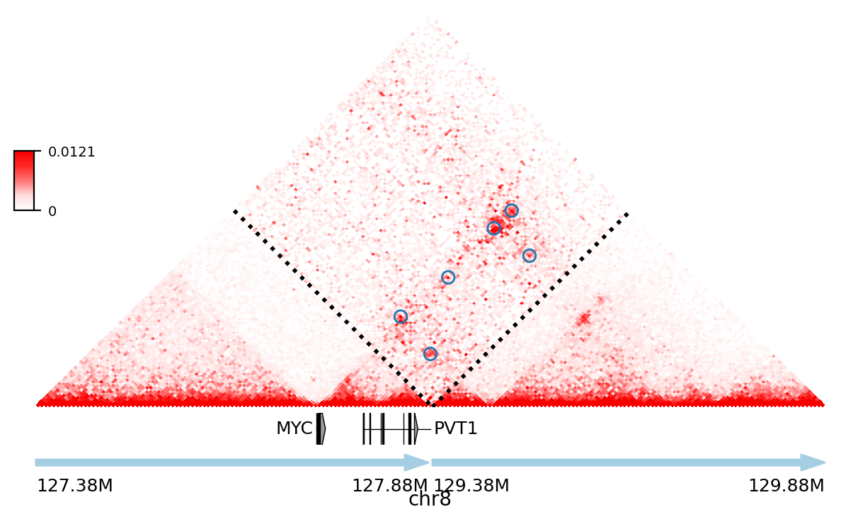
Finally, let's plot the Hi-C matrix, the identified neo-loops, and the gene track on the "C16" assembly, using the built-in visualization module of NeoLoopFinder:
>>> from neoloop.visualize.core import *
>>> import cooler
>>> clr = cooler.Cooler('SKNMC-MboI-allReps-filtered.mcool::resolutions/5000')
>>> assembly = 'C16 deletion,8,127880000,+,8,129375000,-    8,126215000     8,130125000'
>>> vis = Triangle(clr, assembly, n_rows=3, figsize=(7, 4.2),
    track_partition=[5, 0.4, 0.5], correct='sweight', span=500000,
    slopes={(0,0):1, (0,1):0.3, (1,1):1})
>>> vis.matrix_plot(vmin=0)
>>> vis.plot_chromosome_bounds(linewidth=2)
>>> vis.plot_loops('SKNMC.neo-loops.txt', face_color='none', marker_size=40,
    cluster=False, filter_by_res=True, onlyneo=True)
>>> vis.plot_genes(filter_=['MYC', 'PVT1'],label_aligns={'MYC':'right'}, fontsize=9)
>>> vis.plot_chromosome_bar(name_size=10, coord_size=9)
>>> vis.outfig('SKNMC.C16.pdf')
In addtion to the reconstructed Hi-C maps (.cool), loops (.bedpe), and genes, the visualization module also supports plotting RNA-Seq/ChIP-Seq/ATAC-Seq signals (.bigwig), peaks (.bed), and motifs (.bed). Below I'm going to share more examples and the code snippets used to generate the figure.
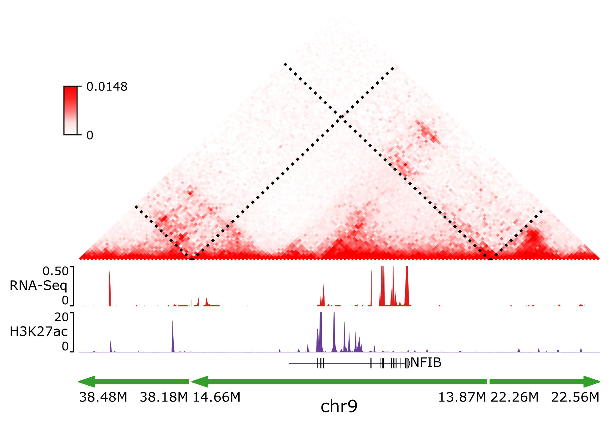
Code Snippet 1:
>>> from neoloop.visualize.core import *
>>> import cooler
>>> clr = cooler.Cooler('SCABER-Arima-allReps.10K.cool')
>>> List = [line.rstrip() for line in open('demo/allOnco-genes.txt')] # please find allOnco-genes.txt in the demo folder of this repository
>>> assembly = 'A3      deletion,9,38180000,-,9,14660000,+      inversion,9,13870000,-,9,22260000,-     9,38480000      9,24220000'
>>> vis = Triangle(clr, assembly, n_rows=5, figsize=(7, 5.2), track_partition=[5, 0.8, 0.8, 0.2, 0.5], correct='weight', span=300000, space=0.08)
>>> vis.matrix_plot(vmin=0, cbr_fontsize=9)
>>> vis.plot_chromosome_bounds(linewidth=2)
>>> vis.plot_signal('RNA-Seq', 'enc_SCABER_RNASeq_rep1.bw', label_size=10, data_range_size=9, max_value=0.5, color='#E31A1C')
>>> vis.plot_signal('H3K27ac', 'SCABER_H3K27ac_pool.bw', label_size=10, data_range_size=9, max_value=20, color='#6A3D9A')
>>> vis.plot_genes(release=75, filter_=List, fontsize=10)
>>> vis.plot_chromosome_bar(name_size=13, coord_size=10)
>>> vis.outfig('SCaBER.NFIB.png', dpi=300)
Figure output 1:
Note that when you initialize a plotting object, the figure size (figsize), the number of tracks (n_rows), and the height of each track (track_partition) can all be configured flexibly.
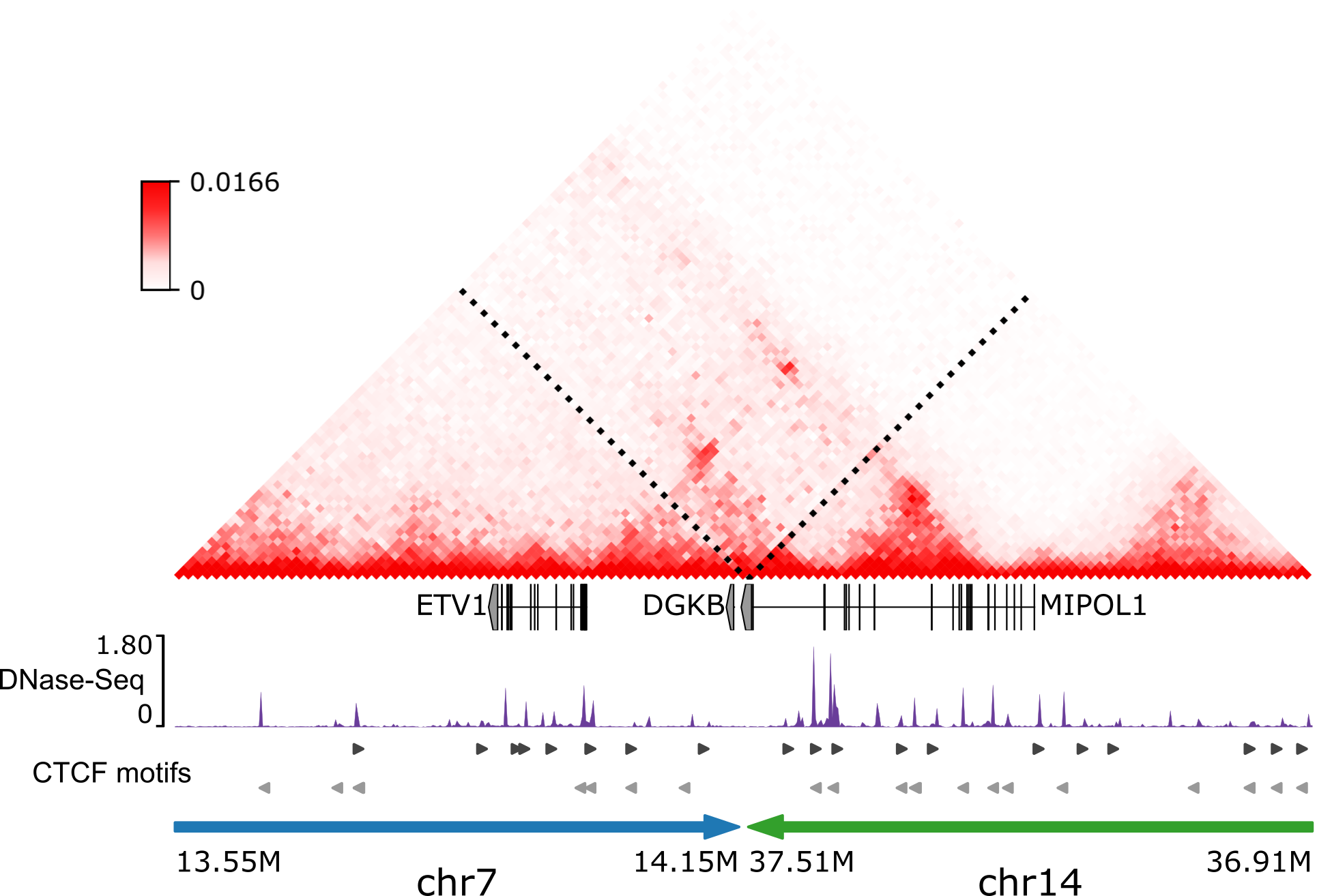
Code Snippet 2:
>>> from neoloop.visualize.core import *
>>> import cooler
>>> clr = cooler.Cooler('LNCaP-WT-Arima-allReps-filtered.mcool::resolutions/10000')
>>> assembly = 'C26     translocation,7,14158275,+,14,37516423,+        7,13140000      14,36390000'
>>> vis = Triangle(clr, assembly, n_rows=6, figsize=(7, 5.3), track_partition=[5, 0.4, 0.8, 0.3, 0.3, 0.5], correct='weight', span=600000, space=0.03)
>>> vis.matrix_plot(vmin=0, cbr_fontsize=9)
>>> vis.plot_chromosome_bounds(linewidth=2)
>>> vis.plot_genes(filter_=['ETV1', 'DGKB', 'MIPOL1'],label_aligns={'DGKB':'right', 'ETV1':'right'}, fontsize=10)
>>> vis.plot_signal('DNase-Seq', 'LNCaP.DNase2.hg38.bw', label_size=10, data_range_size=9, max_value=1.8, color='#6A3D9A')
>>> vis.plot_motif('demo/LNCaP.CTCF-motifs.hg38.txt', subset='+') # an example file LNCaP.CTCF-motifs.hg38.txt can be found at the demo folder of this repository
>>> vis.plot_motif('demo/LNCaP.CTCF-motifs.hg38.txt', subset='-')
>>> vis.plot_chromosome_bar(name_size=13, coord_size=10, color_by_order=['#1F78B4','#33A02C'])
>>> vis.outfig('LNCaP.CTCF-motifs.png', dpi=300)
Figure output 2:
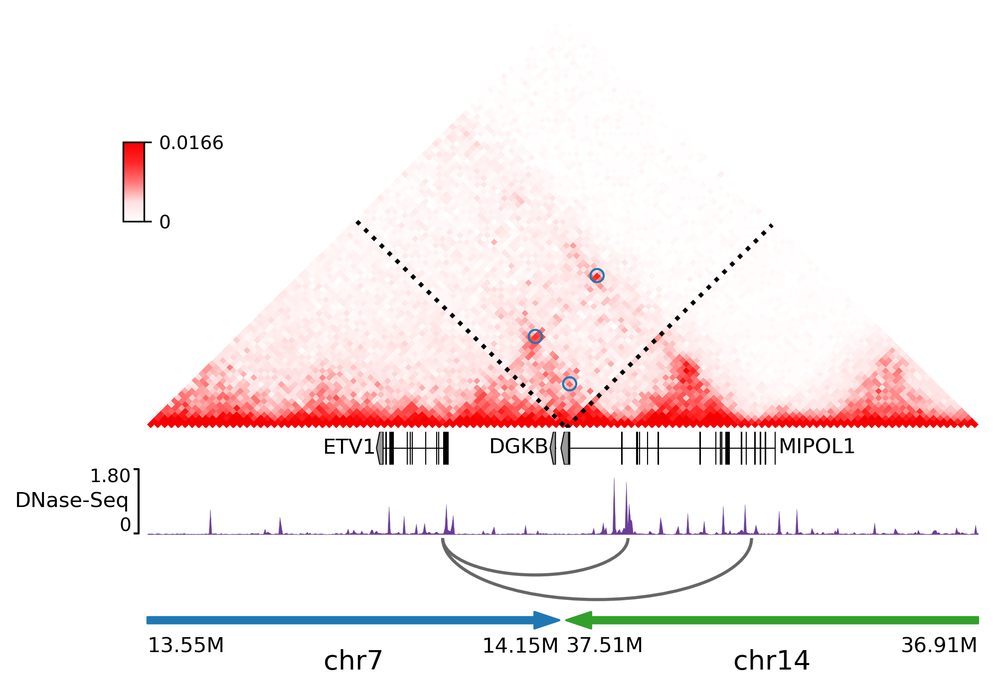
Code Snippet 3:
>>> from neoloop.visualize.core import *
>>> import cooler
>>> clr = cooler.Cooler('LNCaP-WT-Arima-allReps-filtered.mcool::resolutions/10000')
>>> assembly = 'C26     translocation,7,14158275,+,14,37516423,+        7,13140000      14,36390000'
>>> vis = Triangle(clr, assembly, n_rows=5, figsize=(7, 5.3), track_partition=[5, 0.4, 0.8, 0.8, 0.5], correct='weight', span=600000, space=0.03)
>>> vis.matrix_plot(vmin=0, cbr_fontsize=9)
>>> vis.plot_chromosome_bounds(linewidth=2)
>>> vis.plot_loops('LNCaP.neoloops.txt', face_color='none', marker_size=40, cluster=True, onlyneo=True) # only show neo-loops
>>> vis.plot_genes(filter_=['ETV1', 'DGKB', 'MIPOL1'],label_aligns={'DGKB':'right', 'ETV1':'right'}, fontsize=10)
>>> vis.plot_signal('DNase-Seq', 'LNCaP.DNase2.hg38.bw', label_size=10, data_range_size=9, max_value=1.8, color='#6A3D9A')
>>> vis.plot_arcs(lw=1.5, cutoff='top', gene_filter=['ETV1'], arc_color='#666666') # ETV1-related neo-loops
>>> vis.plot_chromosome_bar(name_size=13, coord_size=10, color_by_order=['#1F78B4','#33A02C'])
>>> vis.outfig('LNCaP.arcs.png', dpi=300)
Figure output 3:
Note that both plot_loops and plot_genes need to be called before plot_arcs.
- Made it compatible with the latest versions of dependent packages
- Changed to Peakachu v2.0 models
- Moved all reference data to the 3D genome browser server (http://3dgenome.fsm.northwestern.edu/)
- For CNV segmentation, changed to use the genome-wide CNV profiles to train HMM models
- Made key parameters of the CNV segmentation algorithm tunable


