A library to help:
- model robots and animals which run around and do cool stuff
- run trajectory optimization to understand those models
- animate and plot the results
It's for research into legged critters
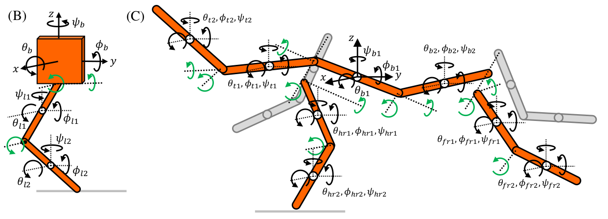
Let's model a monoped hopper, shown in the left on this diagram:
(The complicated quadruped model on the right is where this library starts to shine)
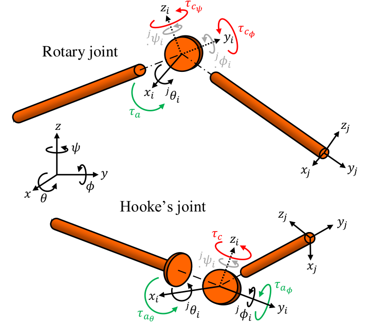
We'll use a rotary joint for the hip (connection between upper link and body) and Hooke's joint for the knee (connection between upper link and lower link), shown in the following diagram:
On to the code:
import physical_education as pe

# create a link called 'base', aligned along the x-axis.
# by default, we use Euler-321 for angle orientation
base = pe.links.Link3D(
    'base', '+x', base=True,
    mass=5., radius=0.4, length=0.4,
)

# we think of this link as starting at the center
# of mass of the base, and pointing downwards (-z)
upper = pe.links.Link3D(
    'upper', '-z', start_I=base.Pb_I,
    mass=.6, radius=0.01, length=0.25,
)

lower = pe.links.Link3D(
    'lower', '-z', start_I=upper.bottom_I,
    mass=.4, radius=0.01, length=0.25,
)

# use an 8-sided polygon for the friction model
pe.foot.add_foot(lower, at='bottom',
                 nsides=8, friction_coeff=1.)

# add relationships between links
# the base has two degrees of freedom with respect
# to the thigh - like a human's hip
base.add_hookes_joint(upper, about='xy')
pe.motor.add_torque(
    base, upper, about='xy',
    torque_bounds=(-2., 2.), no_load_speed=20,
)

# the thigh has one degree of freedom with respect
# to the calf - like a human's knee
upper.add_revolute_joint(lower, about='y')
pe.motor.add_torque(
    upper, lower, about='y',
    torque_bounds=(-2., 2.), no_load_speed=20,
)

# combine into a robot
robot = pe.system.System3D(
    '3D monoped',
    [base, upper, lower],
)

# calculate the equations of motion of the robot
# symbolically, then lambdify them into a regular
# python function
# we'll simplify the equations in parallel, using 8 cores
robot.calc_eom(
    simp_func = lambda x: pe.utils.parsimp(x, nprocs=8),
)
# if you don't want to wait for simplification:
# >>> robot.calc_eom()

# create a pyomo model
# we'll discretize the problem into 50 finite elements,
# use implicit euler for integration, and give a starting
# total time of 1 second whilst allowing individual
# finite elements to vary by +-20%
robot.make_pyomo_model(
    nfe=50, collocation='implicit_euler',
    total_time=1.0, vary_timestep_within=(0.8, 1.2),
)

# let's start with a drop test
# we'll have to write some code, but the idea is that
# this library gives you the tools + example code to
# complete a task. It doesn't have all tasks built in -
# that's what your research is about!
initial_height = 3.0  # meters

nfe = len(robot.m.fe)
ncp = len(robot.m.cp)
body = robot['base']

# start at the origin
body['q'][1, ncp, 'x'].fix(0)
body['q'][1, ncp, 'y'].fix(0)
body['q'][1, ncp, 'z'].fix(initial_height)

# fix initial angle
for link in robot.links:
    for ang in ('phi', 'theta', 'psi'):
        link['q'][1, ncp, ang].fix(0)

# start stationary
for link in robot.links:
    for q in link.pyomo_sets['q_set']:
        link['dq'][1, ncp, q].fix(0)

# initialize to the y plane
for link in robot.links:
    for ang in ('phi', 'theta', 'psi'):
        link['q'][:, :, ang].value = 0

# knee slightly bent at the end
ang = 0.01
upper['q'][nfe, ncp, 'theta'].setlb(ang)
lower['q'][nfe, ncp, 'theta'].setub(-ang)

# but not properly fallen over
body['q'][nfe, ncp, 'z'].setlb(0.2)

# objective: reduce foot penalty (more on that later!)
from pyomo.environ import Objective
pen_cost = pe.foot.feet_penalty(robot)
robot.m.cost = Objective(expr=1000*pen_cost)

# solve! This assumes you have linear solver HSL MA86.
# Let's use L-BGFS, which is _much_ faster for large models
pe.utils.set_ipopt_path('~/CoinIpopt/build/bin/ipopt')
pe.utils.default_solver(
    max_mins=10, solver='ma86',
    OF_hessian_approximation='limited-memory',
).solve(robot.m, tee=True)

# check final penalty value, and so on
robot.post_solve({'penalty': pen_cost})

# animate the result at 1/3 speed, and view along the x-axis
# also, make the camera track the link named 'base'
robot.animate(view_along='x', t_scale=3, track='base')

# let's also view along an elevation of -120 degrees, and
# an azimuth of 35 degrees
robot.animate(view_along=(35, -120), track='base')Larger models benefit tremendously from using PyPy instead of CPython as your python implementation. If you want more clarity on the differences, read this explanation. Anecdotally, PyPy is at least twice as fast when simplifying large models using sympy, and twenty times as fast when setting up models using pyomo. That's the difference of 30 seconds vs 10 minutes!
... which is at times much easier said than done. Instructions are here. You'll also need to install a linear solver. The HSL solvers are the best for many tasks, and their multi-core MA86 solver in particular is very fast. There's a page about HSL + Ipopt, which you should read. This step is usually far easier when done in a Unix environment, like Ubuntu and others like it
If you use a multi-core solver like MA86, you can configure the number of threads to use by setting the OMP_NUM_THREADS environment variable before you launch Python. This can be done on Ubuntu by adding a line like,
# set the number of threads for eg. ma86
OMP_NUM_THREADS=8
to the /etc/environment file, then entering . /etc/environment in a shell or just rebooting. There are other ways of doing this, but due to the way PyOmo runs IPOPT, I've found this to be the easiest and most reliable.
Another way to get the Ipopt binary (plus mumps as a default solver) is by using cyipopt package, which has a super easy installation process (conda install -c conda-forge cyipopt) on Linux and Mac
While you're waiting for things to compile/install, please read this article on supporting black scholars in robotics. All fields (even technical ones, like robotics) are political, and it's crucial that you make an active effort to learn about and combat injustices, such as racism and sexism.
It's recommended that you use a virtual environment - whether that's conda, venv, poetry or whatever else seems easiest to you. This library is on pypi.org, so you should be able to pip install it as follows:
python -m pip install physical_educationIF you use conda, instructions are as follows:
- use pypy, as recommended, now that pypy is available via conda. In the code below, replace
ENV_NAMEwith the name you want to use for your virtual environment:$ conda config --set channel_priority strict $ conda create -c conda-forge --name ENV_NAME pypy $ conda activate ENV_NAME $ pypy3 -m pip install physical_education # see this link for more info: # https://stackoverflow.com/a/62186941/1892669
- or, using CPython:
$ conda create --name ENV_NAME
$ conda activate ENV_NAME
$ conda install pip
$ python -m pip install physical_education
Docs on how to navigate environments can be found here.
Test that it's working:
$ python
>>> import physical_education as pe
>>> pe.visual.success('it worked!')
You can remove an environment using:
$ conda env remove --name ENV_NAMEThat's mentioned in case you eg. try pypy, find it doesn't work, and then want to switch
4. Optional but recommended: install jupyterlab
Jupyterlab is the current version of the Jupyter IDE, which is used to view and run jupyter notebooks. Alex will shamelessly plug his guide on a good setup for this, if you have two computers: a laptop which you want to work on, and a beefy computer where you want optimizations to run
and then start your project. Good luck, and please open an issue if anything is unclear!
outside of commented code/examples, is currently non-existent. I'm finishing off my dissertation now, but intend on working on that afterwards. I have a chapter on this library which serves as a nice intro to everything.

