This is the Repo of my Student Project (Projektarbeit) at the
Biophysics group at the
TU Wien 2021. The final thesis is found as readme.pdf, which acts as
a tutorial for the programs listed here and to analyse the example
data. The described programs roughly divide into the two following
groups:
A Documented walkthrough with examples:
- npc_clustering.ipynb
- npc_clustering.py
 |
 |
A Octave bundle for rigid & affine projections in 3d euclidean space:
- cockpit.m
- ampel.m
- dbscan.m
- rig.m
- affine.m
 |
 |
To begin with, cockpit.m acts as a framework for the entire analysis; successively loading the content of all lokal 2d location files (unless specifically excluded using the exclude variable). All parameters for further analysis are confined to the settings block at the beginning, e.g. load-order corrections due to frames being skipped, etc.
The function ampel.m sorts (modulo) the positions in three categories---red, blue, empty---based on the frame, in which the respective positions have been found by prior localisation. The illumination order (e.g. red-blue-empty) has to stay constant, but the offset (which one of the three staging the starting frame) can, and unfortunately currently has to be adjusted for each file manually by specifying mod values.
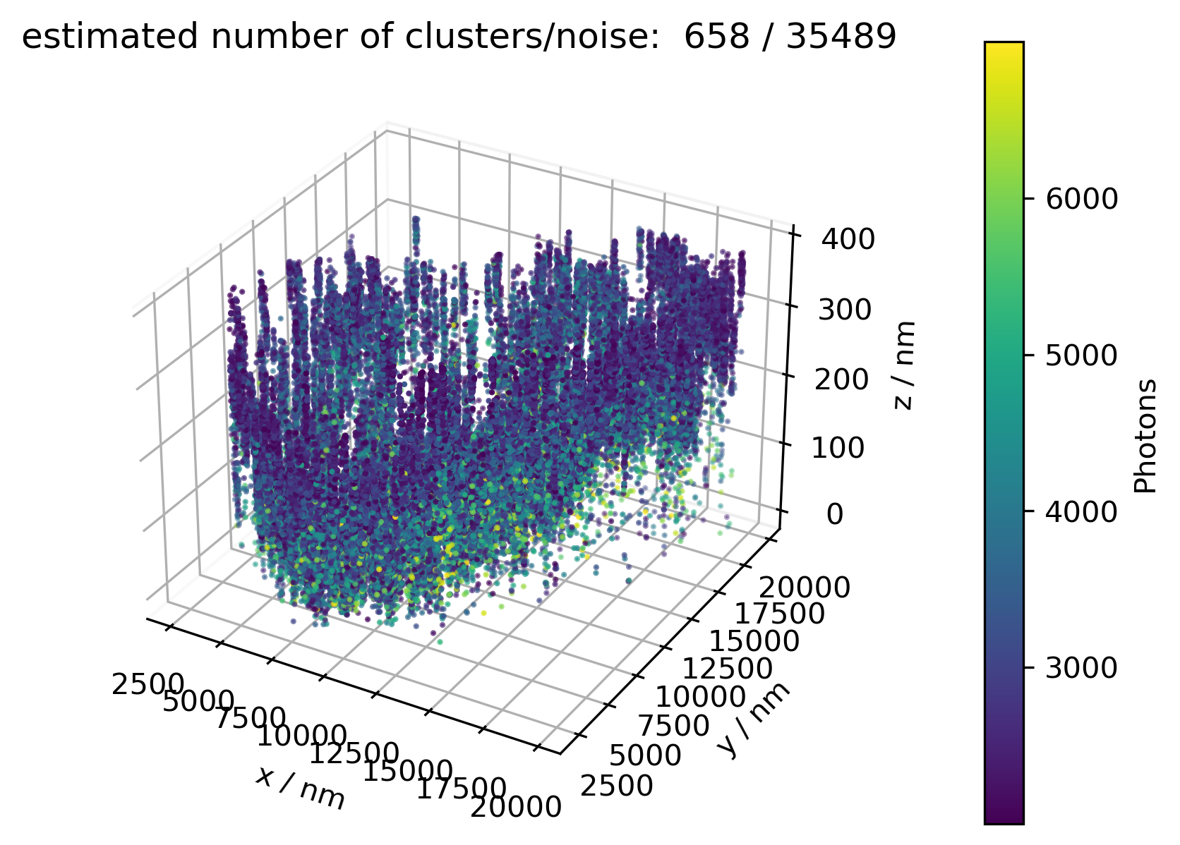
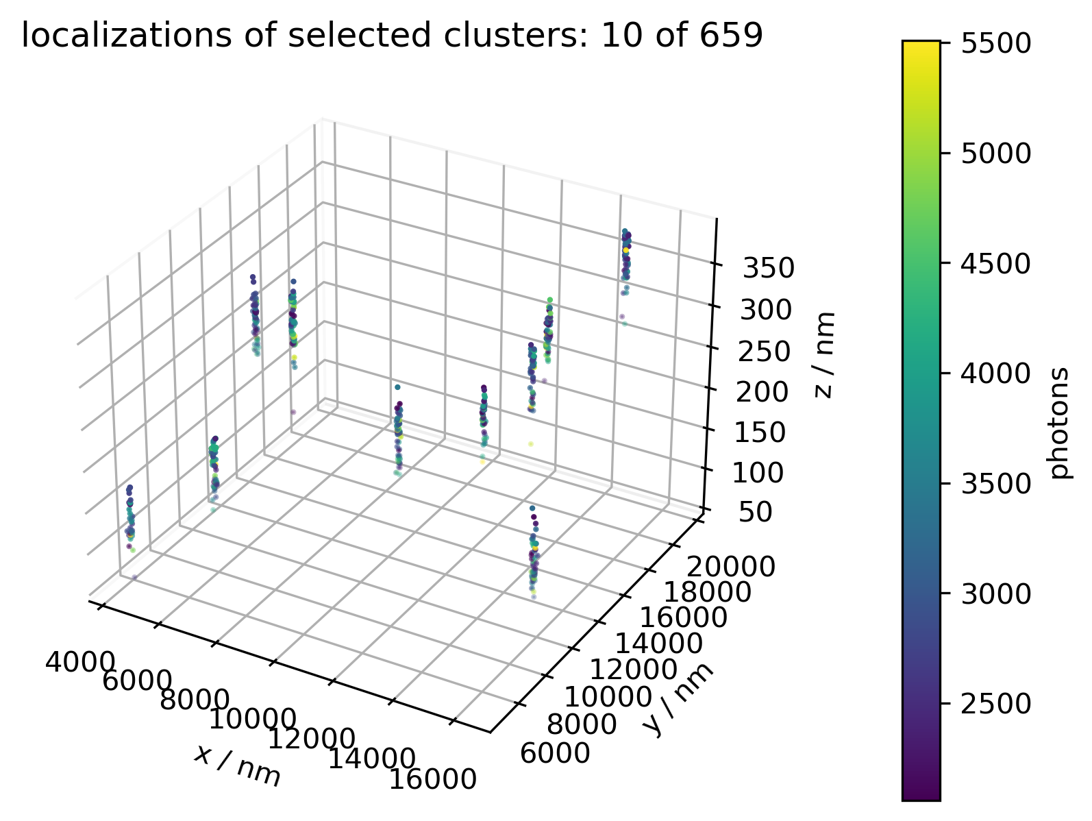
The three separate channels red/blue/empty are then clustered by dbscan.m, based on two parameters: euclidean distance between two neighbours (eps), and least number of points required to be considered a cluster at all (minpts). Based on these parameters, some ensemble of dots are considered a cluster while others are not, which is the whole point of these routines. Naturally, the number of clusters vary with different data sets. Unfortunately though, a rigid projection demands sets of the same size! Brief parameter tuning reveals: Whatever parameters, some regions most likely will have to be excluded. Additionally said clustering takes a long time, due to the slow octave routine; this may be improved by switching to some other (parallel computed) compiled routine. Even worse, clustering generally is very dimension sensitive, so performance is about to drop drastically if we move to 3d!
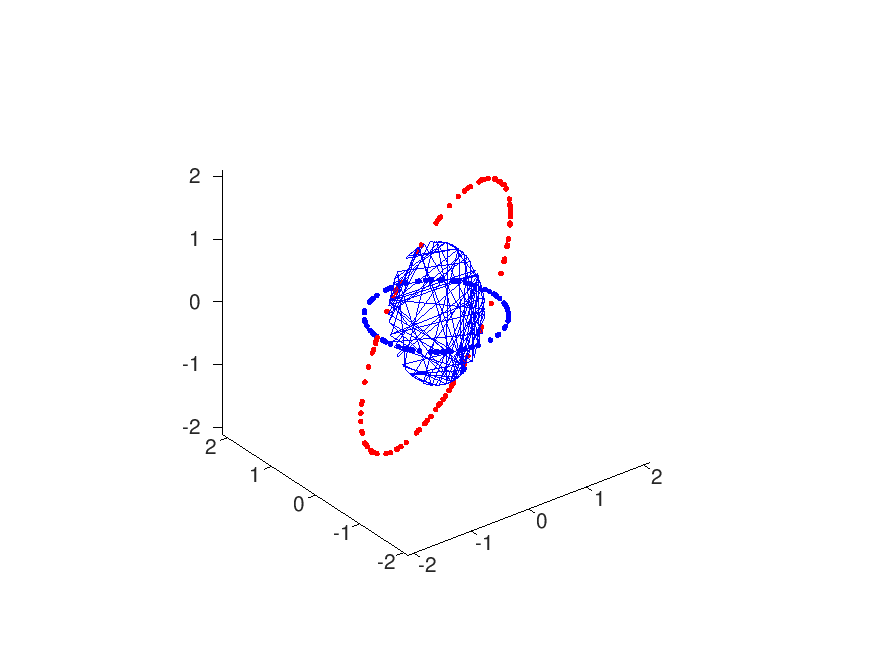
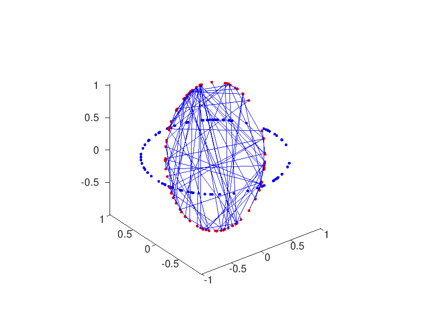
Each of these, say 25, clusters is subsequently approximated by its centroid (arithmetic mean), leaving two sets red/blue of 25 coordinates each. The function rig.m now performs a least squares approximation for the rotation/translation that best projects the blue to the red set. Unfortunately this function does not work in 3d. subsequent statistical analysis on the rotation matrices r and the translation vectors t, of the distinct regions (position files) assert that the red and blue channels are indeed and globally transformed rigidly.
Brief analysis leads to the conclusion that the transformation is somewhat euclidian, but to be honest; the spread (based on mean and standard deviation) is not too great:
- theta = 0.0007 +/- 0.0004 rad
- deltax = 34 +/- 8 nm
- deltay = 29 +/- 4 nm
