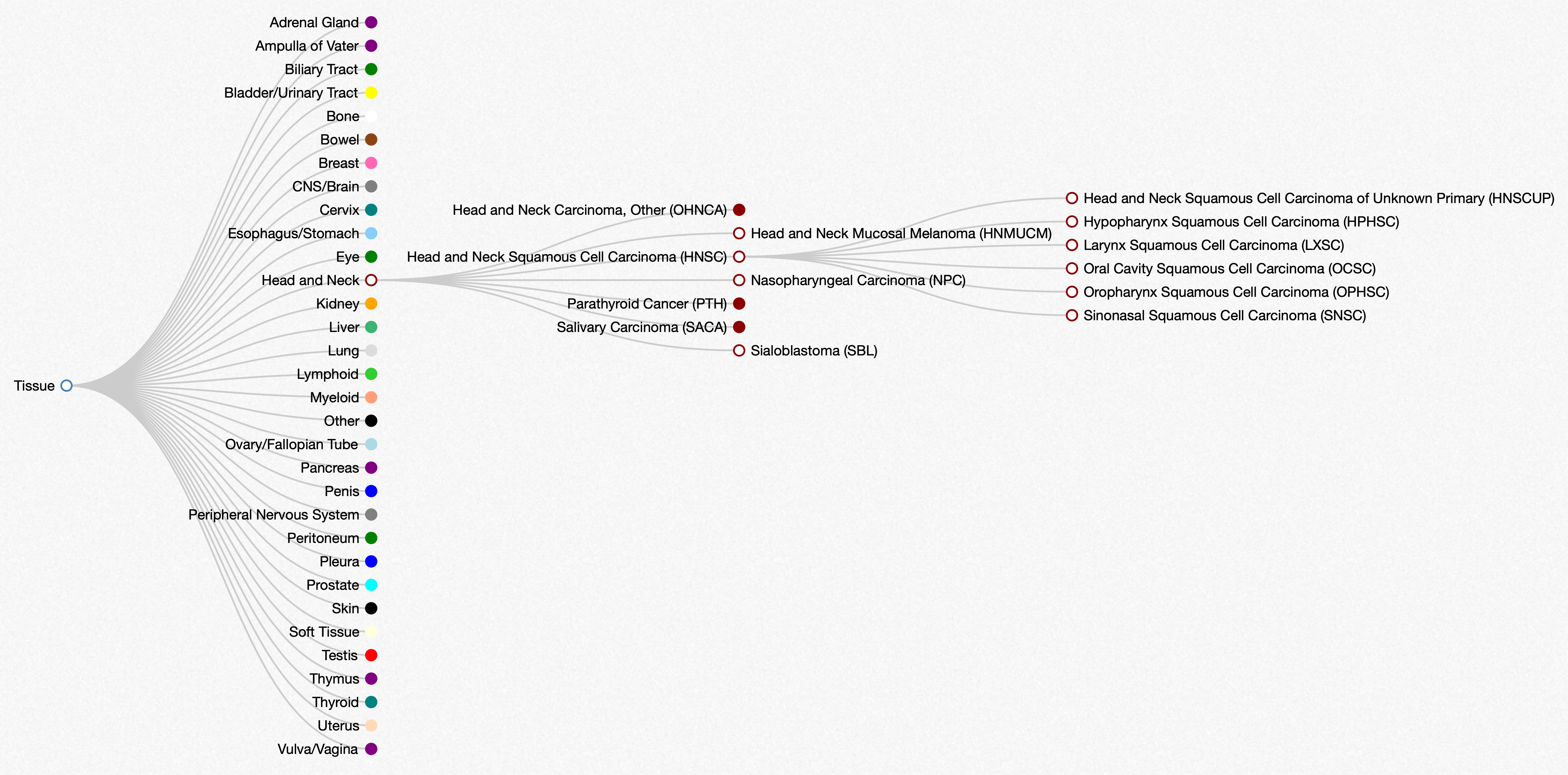
Cancers are often first classified by their tissue of origin, but there are several types of cancer for each tissue. Further, each of these can have several subdivisions. For example, head and neck cancers can be further divided into seven cancers, including head and neck squamous cell carcinoma (HNSC). HNSC itself has six subtypes, too. This hierarchy can be represented in a directed acyclic graph (DAG), as shown below.
The OncoTree is a DAG of cancer subtypes maintained by one of the leading cancer research institutes, Memorial Sloan Kettering (MSK).
For one of my projects in lab, I am dealing with many types of cancers from a variety of studies. Thus, I want to use OncoTree to organize the types and provide relational information of the cancers. For instance, depending on what I want to analyze, I may want the most specific subtype of cancer possible, or maybe I want the cancer grouped by their first level on the OncoTree (e.g. “Head and Neck”).
Therefore, I decided to parse the OncoTree into a ‘tidygraph’, a “tidy” way to manage graph structures. The following is a tutorial on how I did this. The GitHub repository for this analysis is available at jhrcook/tidygraph-oncotree.
I will load the packages ‘tidyverse’, ‘tidygraph’, and ‘ggraph’, and also use ‘httr’ and ‘jsonlite’, but call functions directly from their namespace. The ‘ggraph’ package is a “grammar of graphics” for graph structures - it is used for plotting graphs at the end of this tutorial.
library(ggraph)#> Loading required package: ggplot2
library(tidygraph)#>
#> Attaching package: 'tidygraph'
#> The following object is masked from 'package:stats':
#>
#> filter
library(tidyverse)#> ── Attaching packages ─────────────────────────────────────────────────────── tidyverse 1.2.1 ──
#> ✔ tibble 2.1.3 ✔ purrr 0.3.3
#> ✔ tidyr 1.0.0 ✔ dplyr 0.8.3
#> ✔ readr 1.3.1 ✔ stringr 1.4.0
#> ✔ tibble 2.1.3 ✔ forcats 0.4.0
#> ── Conflicts ────────────────────────────────────────────────────────── tidyverse_conflicts() ──
#> ✖ dplyr::filter() masks tidygraph::filter(), stats::filter()
#> ✖ dplyr::lag() masks stats::lag()
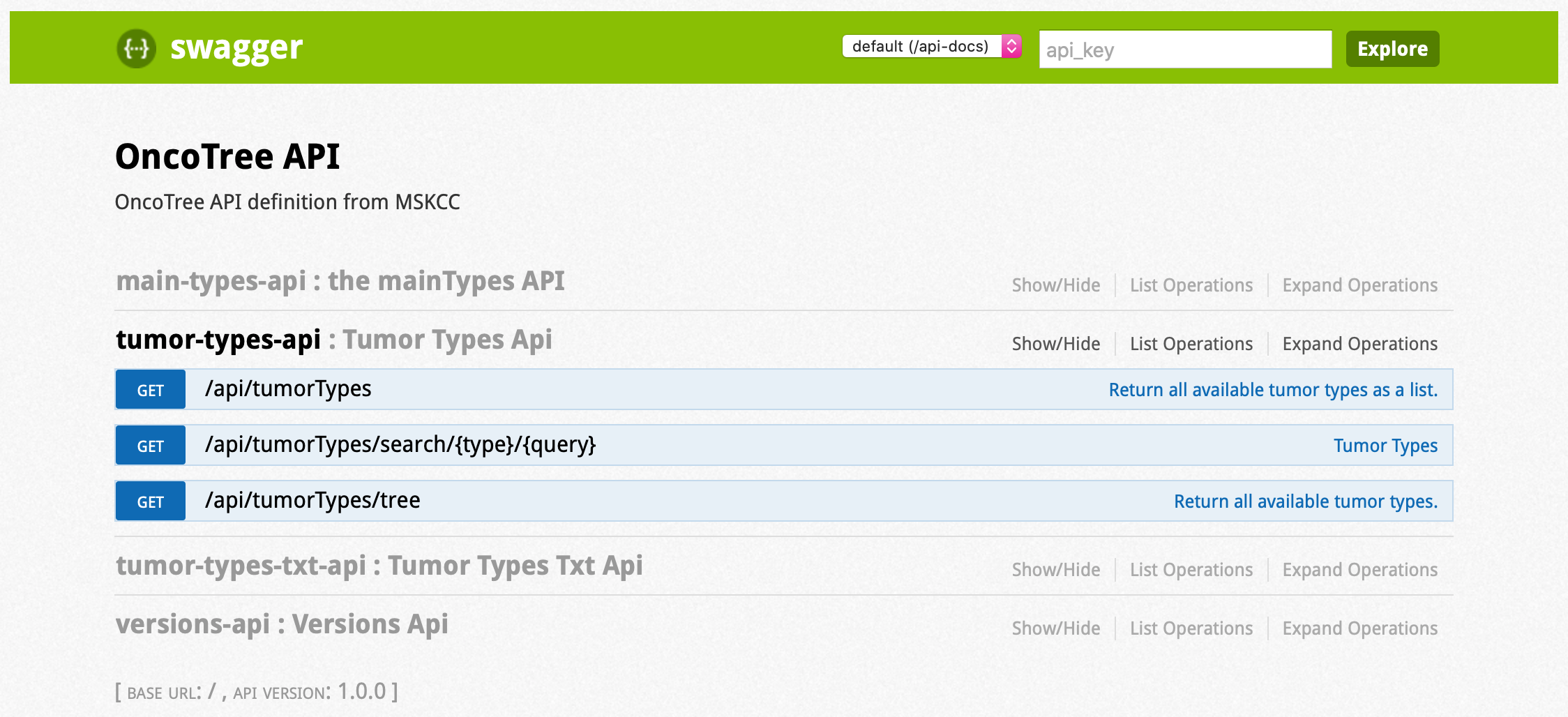
The OncoTree has a fairly simple API (shown below). We are interested in acquiring the full tree so we will use the “/api/tumorTypes/tree” endpoint.
We can use the package ‘httr’ to send a “get” request to the OncoTree API. Checking the status code indicates how the request went, 200 representing success.
oncotree_res <- httr::GET("http://oncotree.mskcc.org/api/tumorTypes/tree")
oncotree_res$status_code
#> [1] 200
The request returns a list of lists containing meta data on the request and the actual OncoTree data.
httr::headers(oncotree_res)#> $date
#> [1] "Mon, 16 Mar 2020 12:59:33 GMT"
#>
#> $server
#> [1] "Apache/2.2.15 (CentOS) mod_jk/1.2.41 mod_ssl/2.2.15 OpenSSL/1.0.1e-fips"
#>
#> $`x-frame-options`
#> [1] "SAMEORIGIN"
#>
#> $vary
#> [1] "Accept-Encoding"
#>
#> $`content-encoding`
#> [1] "gzip"
#>
#> $connection
#> [1] "close"
#>
#> $`transfer-encoding`
#> [1] "chunked"
#>
#> $`content-type`
#> [1] "application/json;charset=UTF-8"
#>
#> attr(,"class")
#> [1] "insensitive" "list"
The OncoTree data is a JSON in the content list of the response. In
case you want this data for other projects, the JSON can be written to
file using the write() function.
write(rawToChar(oncotree_res$content), file.path("oncotree.json"))The OncoTree is organized as a highly nested list. To get insight into the structure we must turn the JSON into a list of lists so we can parse it in R.
oncotree_json <- jsonlite::fromJSON(rawToChar(oncotree_res$content))From here, I just played around with the list until I got an understanding of the structure.
names(oncotree_json)#> [1] "TISSUE"
names(oncotree_json$TISSUE)#> [1] "code" "color" "name"
#> [4] "mainType" "externalReferences" "tissue"
#> [7] "children" "parent" "history"
#> [10] "level" "revocations" "precursors"
oncotree_json$TISSUE$code#> [1] "TISSUE"
oncotree_json$TISSUE$name#> [1] "Tissue"
oncotree_json$TISSUE$level#> [1] 0
Almost all of the parts of oncotree_json$TISSUE contain information
about the first level of the graph. The children section, though,
contains all of the tissues that we can see on the OncoTree web
application.
names(oncotree_json$TISSUE$children)#> [1] "OVARY" "LYMPH" "SOFT_TISSUE" "THYROID"
#> [5] "PLEURA" "PANCREAS" "BILIARY_TRACT" "BREAST"
#> [9] "HEAD_NECK" "EYE" "AMPULLA_OF_VATER" "THYMUS"
#> [13] "CERVIX" "PNS" "BOWEL" "BONE"
#> [17] "SKIN" "BLADDER" "BRAIN" "ADRENAL_GLAND"
#> [21] "PROSTATE" "LUNG" "PENIS" "UTERUS"
#> [25] "OTHER" "TESTIS" "LIVER" "PERITONEUM"
#> [29] "MYELOID" "VULVA" "KIDNEY" "STOMACH"
Each of these children “nodes” had the same information, and children of their own, and so on.
names(oncotree_json$TISSUE$children$HEAD_NECK)#> [1] "code" "color" "name"
#> [4] "mainType" "externalReferences" "tissue"
#> [7] "children" "parent" "history"
#> [10] "level" "revocations" "precursors"
names(oncotree_json$TISSUE$children$HEAD_NECK$children)#> [1] "NPC" "HNMUCM" "PTH" "HNSC" "OHNCA" "SACA" "SBL"
Therefore, we can tell that the JSON is a nested list of the nodes in the DAG. And all we need to do is implement a graph-traversing function to extract all of the information. Since it is nested and we are building a graph, this strongly suggests we will need a recursive algorithm.
To figure out what to do first, I often find it helpful to figure out
what my output should look like. To make a tidygraph, I will need an
edge list and a node list. The first is a two-column table with
names “from” and “to” populated by names of the nodes where each row
indicates an edge of the graph. The node list is optional and contains
any other information about each node, one row per node.
Here is a mock example of the data frames we want out of our recursive algorithm.
# edge list
edge_list <- tibble::tribble(
    ~ from, ~ to,
       "A",  "B",
       "B",  "C",
       "C",  "D",
       "A",  "D",
       "B",  "E",
       "E",  "D"
)
edge_list
#> # A tibble: 6 x 2
#> from to
#> <chr> <chr>
#> 1 A B
#> 2 B C
#> 3 C D
#> 4 A D
#> 5 B E
#> 6 E D
# node list
node_list <- tibble(name = LETTERS[1:5], values = round(runif(5), 2))
node_list
#> # A tibble: 5 x 2
#> name values
#> <chr> <dbl>
#> 1 A 0.04
#> 2 B 0.81
#> 3 C 0.35
#> 4 D 0.580
#> 5 E 0.97
The edge list can be turned into a tidygraph object using the
as_tbl_graph() function. I explicitly set the directed parameter
TRUE even though it is the default value.
gr <- as_tbl_graph(edge_list, directed = TRUE)
gr
#> # A tbl_graph: 5 nodes and 6 edges
#> #
#> # A directed acyclic simple graph with 1 component
#> #
#> # Node Data: 5 x 1 (active)
#> name
#> <chr>
#> 1 A
#> 2 B
#> 3 C
#> 4 E
#> 5 D
#> #
#> # Edge Data: 6 x 2
#> from to
#> <int> <int>
#> 1 1 2
#> 2 2 3
#> 3 3 5
#> # … with 3 more rows
To add the node information, I join the node list table by the “name”
column. The %N>% infix operates just like the ‘magrittr’ pipe %>%
except it also activates the nodes of the tidygraph object so that the
full_join() operates on the nodes and not the edges. I am not able to
fully describe the ‘tidygraph’ API in this tutorial, but see vignettes
by the creator, Thomas Pedersen
(@thomasp85), for a good introduction:
Data Imaginist -
tidygraph.
gr %N>%
    full_join(node_list, by = "name")
#> # A tbl_graph: 5 nodes and 6 edges
#> #
#> # A directed acyclic simple graph with 1 component
#> #
#> # Node Data: 5 x 2 (active)
#> name values
#> <chr> <dbl>
#> 1 A 0.04
#> 2 B 0.81
#> 3 C 0.35
#> 4 E 0.97
#> 5 D 0.580
#> #
#> # Edge Data: 6 x 2
#> from to
#> <int> <int>
#> 1 1 2
#> 2 2 3
#> 3 3 5
#> # … with 3 more rows
Now we just need to figure out how to build an edge list and node list from the nested JSON.
Note: Below I demonstrate how to create the final algorithm as if it was a linear process - it in fact took me about and hour and a half of toying with the functions to get the desired result. If it is not easy to grasp right away, don’t worry, it wasn’t for me either.
So we know our algorithm will be recursive, which means we will pass the
first node to a function once and this function will call itself from
within. Therefore, let’s create a function add_children_to_dag() that
takes a node and an edge list and returns an edge list.
add_children_to_dag <- function(node, el) {
    return(el)
}First, we can deal with the node information becasue that can be extracted right away and stashed in a global variable, no recursion needed.
# The node information.
NODE_INFO <- tibble()

# Build a tibble of the node information from Oncotree.
extract_node_info <- function(node) {
    NODE_INFO <<- bind_rows(
        NODE_INFO,
        tibble(
            code = node$code,
            description = node$name,
            tissue = ifelse(is.null(node$tissue), "tissue", node$tissue),
            main_type = ifelse(is.null(node$mainType), "tissue", node$mainType),
            color = ifelse(is.null(node$color), "Black", node$color),
            level = node$level
        )
    )
}


add_children_to_dag <- function(node, el) {
    # Add node information to the `NODE_INFO` global variable.
    extract_node_info(node)

    return(el)
}
Now, the node information is extracted and added to a global variable
NODE_INFO using the extract_node_info() function. It just pulls out
some of the useful information from the JSON for each node and binds it
with the existing data frame.
Now we can run the first experiment to make sure everything is working
properly. The initial edge list is just an empty tibble().
add_children_to_dag(oncotree_json[[1]], tibble())#> # A tibble: 0 x 0
Nothing is done to the el variable in add_children_to_dag() function
yet, so it returns an empty data frame. However, the NODE_INFO data
frame should have the information for the first level of OncoTree.
NODE_INFO#> # A tibble: 1 x 6
#> code description tissue main_type color level
#> <chr> <chr> <chr> <chr> <chr> <int>
#> 1 TISSUE Tissue tissue tissue Black 0
Success!
Now we need to start on the hard part, the recursive traversal of the
DAG in the JSON. To begin, we should add an if-statement to check if the
node has children. If it does, then we need to add the connections from
this node to the children to the edge list el.
This is easily done by binding the existing el with a new tibble with
“from” and “to” columns containing the name of the current node (from)
and the names of the children (to).
Let’s start with that and make sure it works.
add_children_to_dag <- function(node, el) {
    # Add node information to the `NODE_INFO` global variable.
    extract_node_info(node)

    if (length(names(node$children)) > 0) {
        # Add this node and children to edge list.
        el <- bind_rows(el, tibble(from = node$code, to = names(node$children)))
    }
    return(el)
}add_children_to_dag(oncotree_json[[1]], tibble())#> # A tibble: 32 x 2
#> from to
#> <chr> <chr>
#> 1 TISSUE OVARY
#> 2 TISSUE LYMPH
#> 3 TISSUE SOFT_TISSUE
#> 4 TISSUE THYROID
#> 5 TISSUE PLEURA
#> 6 TISSUE PANCREAS
#> 7 TISSUE BILIARY_TRACT
#> 8 TISSUE BREAST
#> 9 TISSUE HEAD_NECK
#> 10 TISSUE EYE
#> # … with 22 more rows
Great! We can see that the connections from "TISSUE" to each of the
top-level cancer groups were successfully added to the edge list.
Now we need to apply this function to each of the children of this node.
I do this with map() from the ‘purrr’ package (attached along with
‘tidyverse’). It works similarly to lapply() from base R, but is a
bit easier to manage, in my opinon (and it has some other useful helpers
and capabilities that we don’t use here.)
Basically, each child node is passed to add_children_to_dag() along
with the edge list. The node information for each child will be
extracted and, if they have children, they will be sent through
add_children_to_dag(), too. Each time, an edge list is returned.
This is a recursive process and will naturally visit every node, building up the edge list through every “leaf” on the tree.
add_children_to_dag <- function(node, el) {
    # Add node information to the `NODE_INFO` global variable.
    extract_node_info(node)

    if (length(names(node$children)) > 0) {
        # Add this node and children to edge list.
        nodes_el <- bind_rows(el, tibble(from = node$code, to = names(node$children)))

        # Repeat for children nodes.
        childrens_el <- map(node$children, add_children_to_dag, el = el)

        # Combine into one edge list.
        el <- bind_rows(nodes_el, childrens_el)
    }
    return(el)
}
And that’s it! We should now be able to create the entire DAG.
# reset `NODE_INFO`
NODE_INFO <- tibble()

# Run the recursive algorithm.
oncotree_el <- add_children_to_dag(oncotree_json[[1]], tibble())
oncotree_el
#> # A tibble: 867 x 2
#> from to
#> <chr> <chr>
#> 1 TISSUE OVARY
#> 2 TISSUE LYMPH
#> 3 TISSUE SOFT_TISSUE
#> 4 TISSUE THYROID
#> 5 TISSUE PLEURA
#> 6 TISSUE PANCREAS
#> 7 TISSUE BILIARY_TRACT
#> 8 TISSUE BREAST
#> 9 TISSUE HEAD_NECK
#> 10 TISSUE EYE
#> # … with 857 more rows
NODE_INFO#> # A tibble: 868 x 6
#> code description tissue main_type color level
#> <chr> <chr> <chr> <chr> <chr> <int>
#> 1 TISSUE Tissue tissue tissue Black 0
#> 2 OVARY Ovary/Fallopian Tube Ovary/Fall… Ovarian/Fallopian… Light… 1
#> 3 OOVC Ovarian Cancer, Other Ovary/Fall… Ovarian Cancer Light… 2
#> 4 OCNOS Ovarian Choriocarcinoma, … Ovary/Fall… Ovarian Cancer Light… 3
#> 5 HGONEC High-Grade Neuroendocrine… Ovary/Fall… Ovarian Cancer Light… 3
#> 6 HGSFT High-Grade Serous Fallopi… Ovary/Fall… Ovarian Cancer Light… 3
#> 7 OVT Ovarian Epithelial Tumor Ovary/Fall… Ovarian Cancer Light… 2
#> 8 EBOV Endometrioid Borderlin Ov… Ovary/Fall… Ovarian Cancer Light… 3
#> 9 SOC Serous Ovarian Cancer Ovary/Fall… Ovarian Cancer Light… 3
#> 10 HGSOC High-Grade Serous Ovarian… Ovary/Fall… Ovarian Cancer Light… 4
#> # … with 858 more rows
Just as before, the tidygraph object can be constructed from the edge
list, followed by joining the node list information.
oncotree_gr <- as_tbl_graph(oncotree_el, directed = TRUE) %N>%
    full_join(NODE_INFO, by = c("name" = "code"))
This tidygraph object can now be saved for future reference.
saveRDS(oncotree_gr, "msk_oncotree_tidygraph.rds")To make the visualization a bit better, I mapped the colors extracted from the JSON to colors available in R.
oncotree_colors <- tibble::tribble(
             ~ color,      ~ new_color,
             "black",          "black",
             "Black",          "black",
              "Blue",           "blue",
              "Cyan",           "cyan",
           "DarkRed",        "darkred",
         "Gainsboro",        "#DCDCDC",
              "Gray",           "grey",
             "Green",          "green",
           "HotPink",        "hotpink",
         "LightBlue",      "lightblue",
       "LightSalmon",    "lightsalmon",
      "LightSkyBlue",   "lightskyblue",
       "LightYellow",    "lightyellow",
         "LimeGreen",      "limegreen",
    "MediumSeaGreen", "mediumseagreen",
            "Orange",         "orange",
         "PeachPuff",        "#FFDAB9",
            "Purple",         "purple",
               "Red",            "red",
       "SaddleBrown",           "tan4",
              "Teal",        "#008080",
             "White",          "white",
            "Yellow",         "yellow"
)

oncotree_gr <- oncotree_gr %N>%
    left_join(oncotree_colors, by = "color") %>%
    select(-color) %>%
    dplyr::rename(color = new_color)
Finally, we can use the ‘ggraph’ package to create some visualizations of the DAG. Again, I am unable to fully explain ‘ggraph’ here, but the package vignettes are very good: Data Imaginist - ggraph.
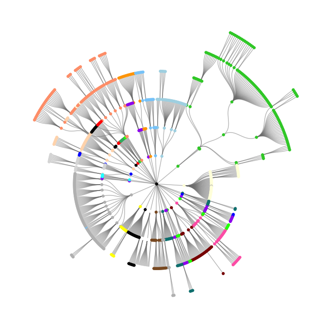
The first plot below shows the OncoTree graph spreading radially from the center, each layer representing a further subdivision of the cancer type. The colors roughly correspond to the tissue of origin.
oncotree_gr %N>%
    ggraph(layout = "tree", circular = TRUE) +
    geom_edge_diagonal(color = "grey50", alpha = 0.5) +
    geom_node_point(aes(color = color)) +
    scale_color_identity() +
    theme_graph()
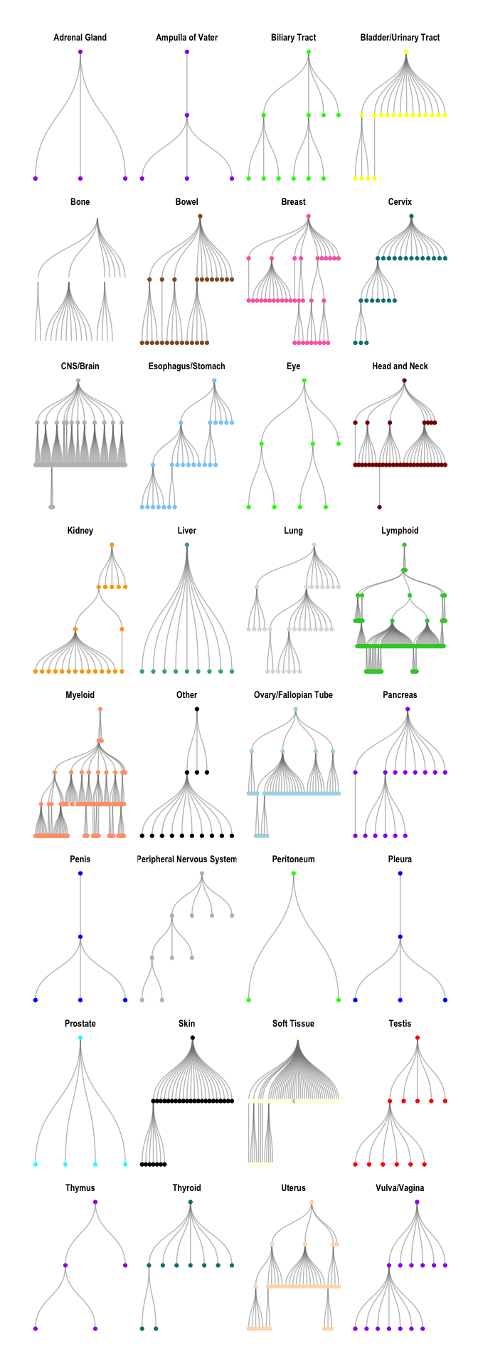
Each of the subgraphs can also be separated by tissue of origin.
oncotree_gr %N>%
    filter(name != "TISSUE") %>%
    morph(to_components) %>%
    mutate(grp = tissue[which.max(level)]) %>%
    unmorph() %>%
    ggraph(layout = "tree") +
    facet_nodes(~ grp, ncol = 4, scales = "free") +
    geom_edge_diagonal(color = "grey50", alpha = 0.5) +
    geom_node_point(aes(color = color)) +
    scale_color_identity() +
    theme_graph()
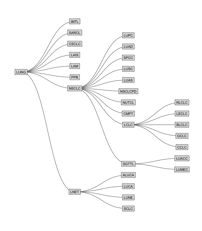
And below is an example of the subdivisions of lung cancer.
oncotree_gr %N>%
    filter(name != "TISSUE") %>%
    morph(to_components) %>%
    mutate(grp = tissue[which.max(level)]) %>%
    unmorph() %N>%
    filter(grp == "Lung") %>%
    ggraph(layout = "tree") +
    geom_edge_diagonal(color = "grey50") +
    geom_node_label(aes(label = name, fill = color), size = 3,
                    repel = FALSE, label.r = unit(0.1, "lines")) +
    scale_fill_identity() +
    coord_flip() +
    scale_y_reverse() +
    theme_graph()