In this project, your goal is to write a software pipeline to identify the lane boundaries in a video, but the main output or product we want you to create is a detailed writeup of the project. Check out the writeup template for this project and use it as a starting point for creating your own writeup.
A great writeup should include the rubric points as well as your description of how you addressed each point. You should include a detailed description of the code used in each step (with line-number references and code snippets where necessary), and links to other supporting documents or external references. You should include images in your writeup to demonstrate how your code works with examples.
All that said, please be concise! We're not looking for you to write a book here, just a brief description of how you passed each rubric point, and references to the relevant code :).
You're not required to use markdown for your writeup. If you use another method please just submit a pdf of your writeup.
The goals / steps of this project are the following:
- Compute the camera calibration matrix and distortion coefficients given a set of chessboard images.
- Apply a distortion correction to raw images.
- Use color transforms, gradients, etc., to create a thresholded binary image.
- Apply a perspective transform to rectify binary image ("birds-eye view").
- Detect lane pixels and fit to find the lane boundary.
- Determine the curvature of the lane and vehicle position with respect to center.
- Warp the detected lane boundaries back onto the original image.
- Output visual display of the lane boundaries and numerical estimation of lane curvature and vehicle position.
See my video_result_demo on youtube.
Note: all python files(except for the python class Lane_class.py) can run separately. You can also see my jupyter notebook Advanced_lane_detection.ipynb for more visual results.
1. Provide a Writeup / README that includes all the rubric points and how you addressed each one. You can submit your writeup as markdown or pdf. Here is a template writeup for this project you can use as a guide and a starting point.
You're reading it!
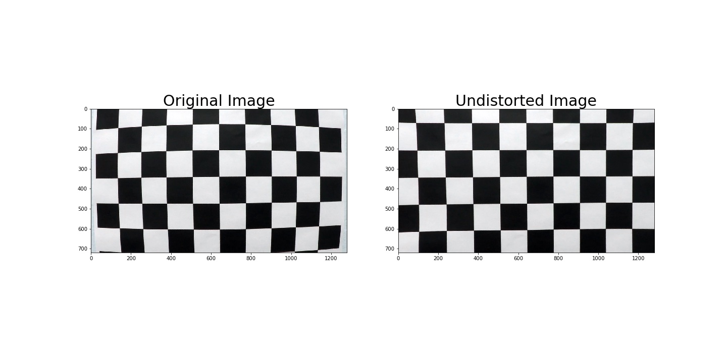
1. Briefly state how you computed the camera matrix and distortion coefficients. Provide an example of a distortion corrected calibration image.
The code for this step is contained in camera_calibration.py, you can also find them in jupyter notebook code cell 3-4.
We use ./camera_cal*.jpg to calibrate the camera.
-
Convert to grayscale.
-
Use cv2.findChessboardCorners and cv2.calibrateCamera to calibrate images
-
Use cv2.undistort to undist images
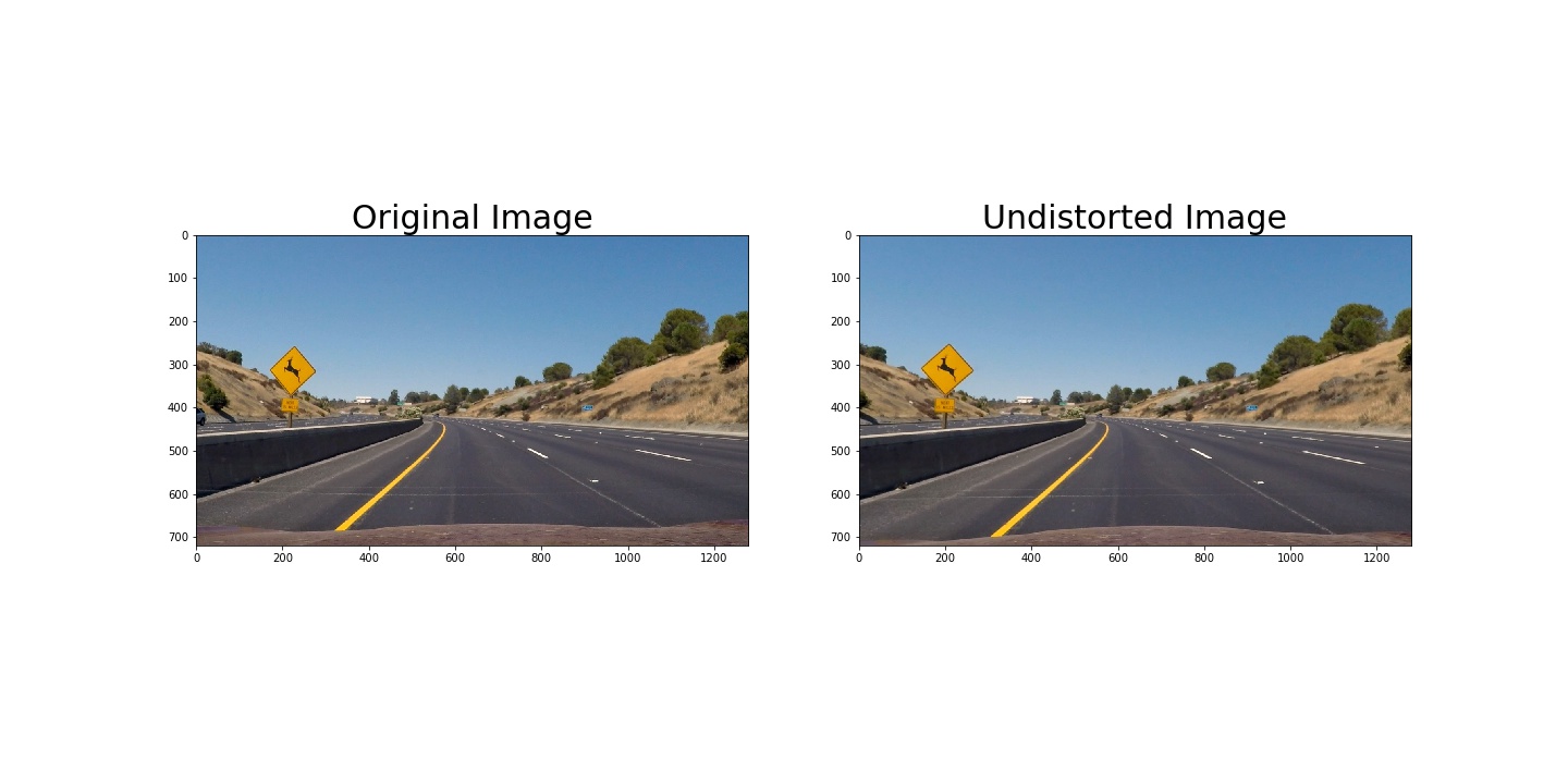
We also save parameters for later use. Here is one example of the results:
To demonstrate this step, I will describe how I apply the cameral calibration and distortion correction to one of the test images like this one:
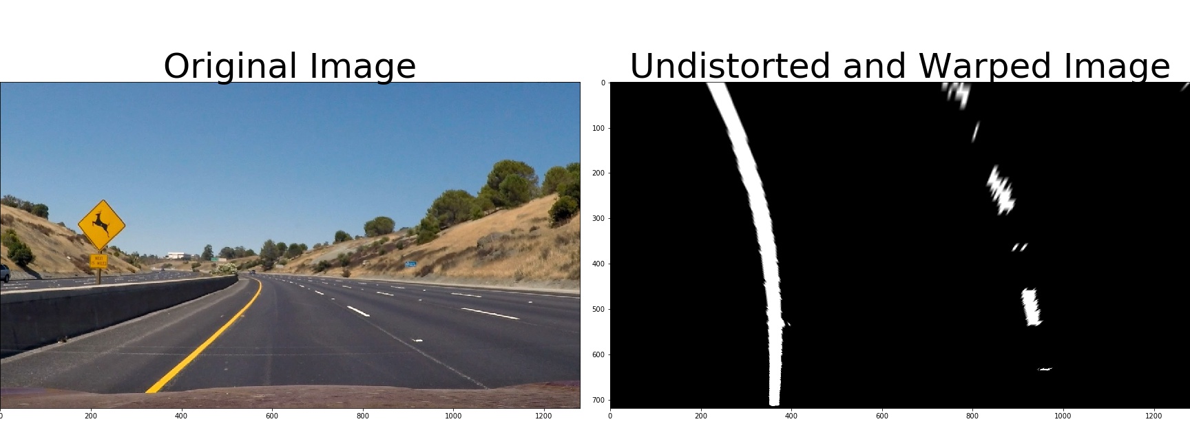
2. Describe how (and identify where in your code) you used color transforms, gradients or other methods to create a thresholded binary image. Provide an example of a binary image result.
The code for this step is contained in combined_thresh.py, you can also find them in jupyter notebbok code cell 7.
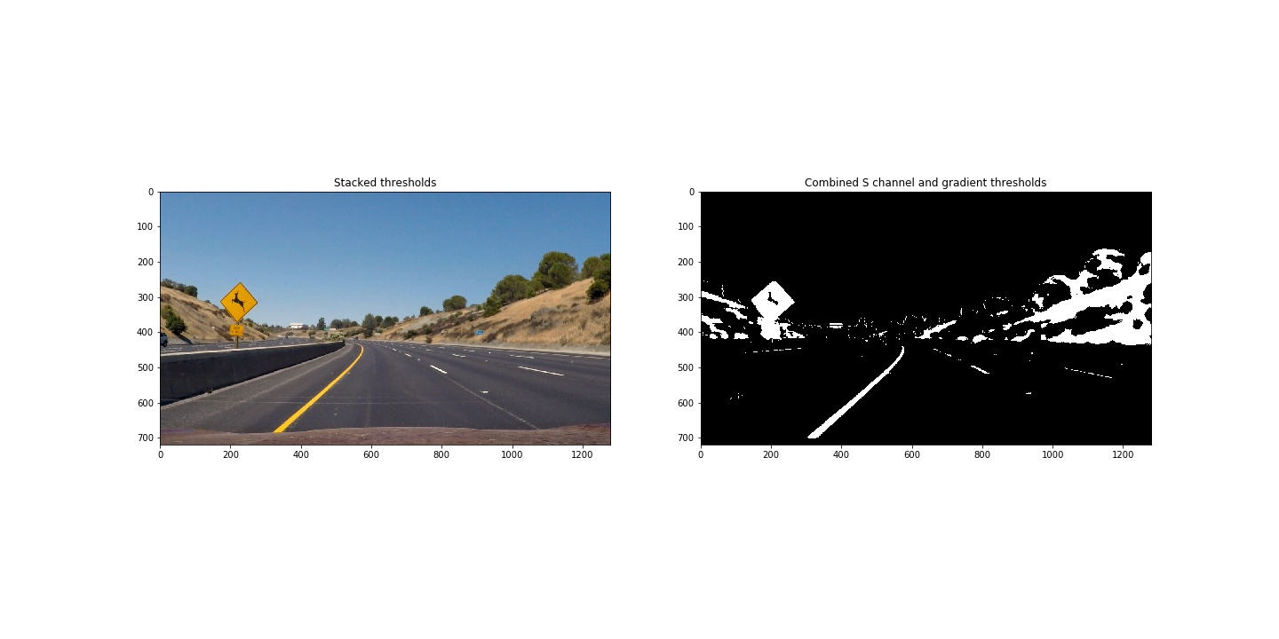
I used a combination of color and gradient thresholds to generate a binary image. Here's an example of my output for this step.
-
Absolute sobel operator in x direction
-
Magnitude sobel oprator for combined x direction and y direction
-
Direction gradient sobel operator for y direction versus x direction
-
Use S chanel of HLS color space since it can strength yellow lines while grayscale perform bad on yellow lines.
-
Use YUV color space. Pixels with a V component less than 105 are deemed white, while pixels with a Y component greater than or equal to 205 are deemed yellow
Here is the combined threshold applyed to one of the test image like this one:
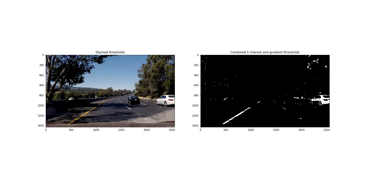
Here is the combined threshold applyed to another one of the test image with sharp road and heavy shadows like this one:
3. Describe how (and identify where in your code) you performed a perspective transform and provide an example of a transformed image.
The code for this step can be found in Perspective_transform.py, you can also find them in jupyter notebook code cell 9.
-
Define source(
src) and destination(dst) -
Use cv2.getPerspectiveTransform(src, dst) to calculate the perspective transform matrix
-
Use cv2.warpPerspective to warped the image
I also use cv2.getPerspectiveTransform(dst, src) to calculate inversed perspective transorm matrix for later use. For the source (src) and destination (dst) points. I chose the the source and destination points in the following manner by hands:
| Source | Destination |
|---|---|
| 200, img_size[1] | 300, img_size[1] |
| 1200, img_size[1] | 960, img_size[1] |
| 700, 450 | 960, 0 |
| 585, 450 | 300, 0 |
However, I will try to hardcode the source and destination points like the following manner since this way is more robust:
src = np.float32(
    [[(img_size[0] / 2) - 55, img_size[1] / 2 + 100],
    [((img_size[0] / 6) - 10), img_size[1]],
    [(img_size[0] * 5 / 6) + 60, img_size[1]],
    [(img_size[0] / 2 + 55), img_size[1] / 2 + 100]])
dst = np.float32(
    [[(img_size[0] / 4), 0],
    [(img_size[0] / 4), img_size[1]],
    [(img_size[0] * 3 / 4), img_size[1]],
    [(img_size[0] * 3 / 4), 0]])
I verified that my perspective transform was working as expected by drawing the src and dst points onto a test image and its warped counterpart to verify that the lines appear parallel in the warped image.
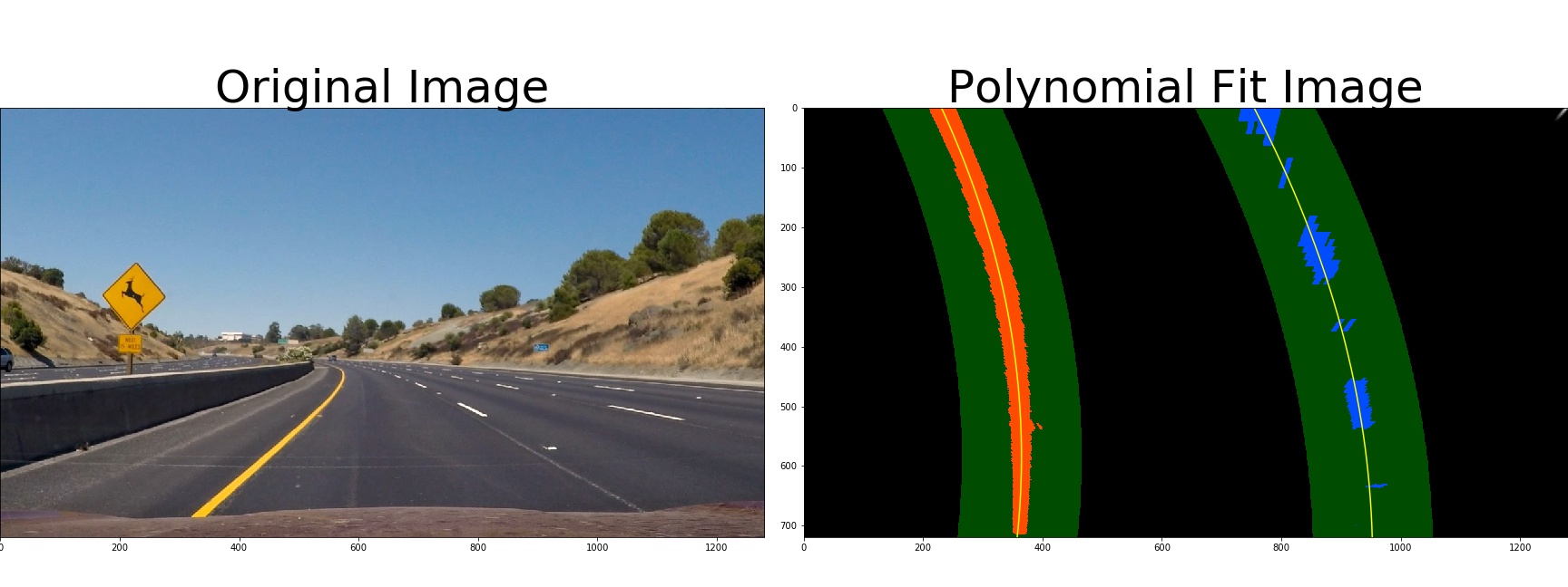
4. Describe how (and identify where in your code) you identified lane-line pixels and fit their positions with a polynomial?
The code for this step is contained in polynomial_fit.py, you can also find them in jupyter notebook code cell 23
After applying calibration, thresholding, and a perspective transform to a road image, we have a binary warped image where the lane lines stand out clearly. However, we still need to decide explicitly which pixels are part of the lines and which belong to the left line and which belong to the right line.
I use a histogram to find the peaks of the binary warped image. The code is defined as line_fit function in code lines 16-119 of polynomial_fit.py, visualization for this function defined as line_fit_visualize function in lines 121-144 of polynomial_fit.py. Steps like this:
We then can slide window to find the left lane and right lane.
-
Find the peak of the left and right halves of the histogram
-
Choose a number of sliding windows, here is 9
-
Step through the windows one by one to update current positions for each window
-
Identify and extract left and right line pixel positions
-
Fit a second order polynomial to each
Once we know where the lines are we have a fit! In the next frame of video we don't need to do a blind search again, but instead we can just search in a margin around the previous line position. The code is defined as advanced_fit function in code lines 148-220 of polynomial_fit.py, visualization for this function defined as advanced_fit_visualize function in lines 222-265 of polynomial_fit.py.
Note both line_fit and advanced_fit, I check whether we find enough points, If I don't get not enough points, return None with error.
Here is the Polynomial fit applyed to one of the test image like this one
5. Describe how (and identify where in your code) you calculated the radius of curvature of the lane and the position of the vehicle with respect to center.
The code for this step is contained in Curvature_offset_process_video.py, you can also find them in jupyter notebook code cell 29-32.
-
Calculate
curvaturefor left lane and right lane according to equations. -
Converts curvature from pixes to meters. Assume the lane is about 30 meters long(per 720 pixels) and 3.7 meters wide(per 700 pixes) according to the U.S. government specifications for highway curvature.
-
Calculate
vehicle offsetof the lane center from the center of the image. I use the average of left lane and right lane minus the lane center as the offset. If the offset is larger than 0, the vehicle is right offset from lane center. If the offset is smaller than 0, the vehicle is left offset from lane center -
Anotate information of curvature and vehicle offset in the original undistorted image The code for calculating curvature is defined as
calculate_curvature functionin code lines 18-37 ofCurvature_offset_process_video.py. The code for calculating vehicle is defined ascalculate_offset functionin code lines 39-50 ofCurvature_offset_process_video.py. The code for anotating informations is defined asfinal_drawing functionin code lines 52-92Curvature_offset_process_video.py.
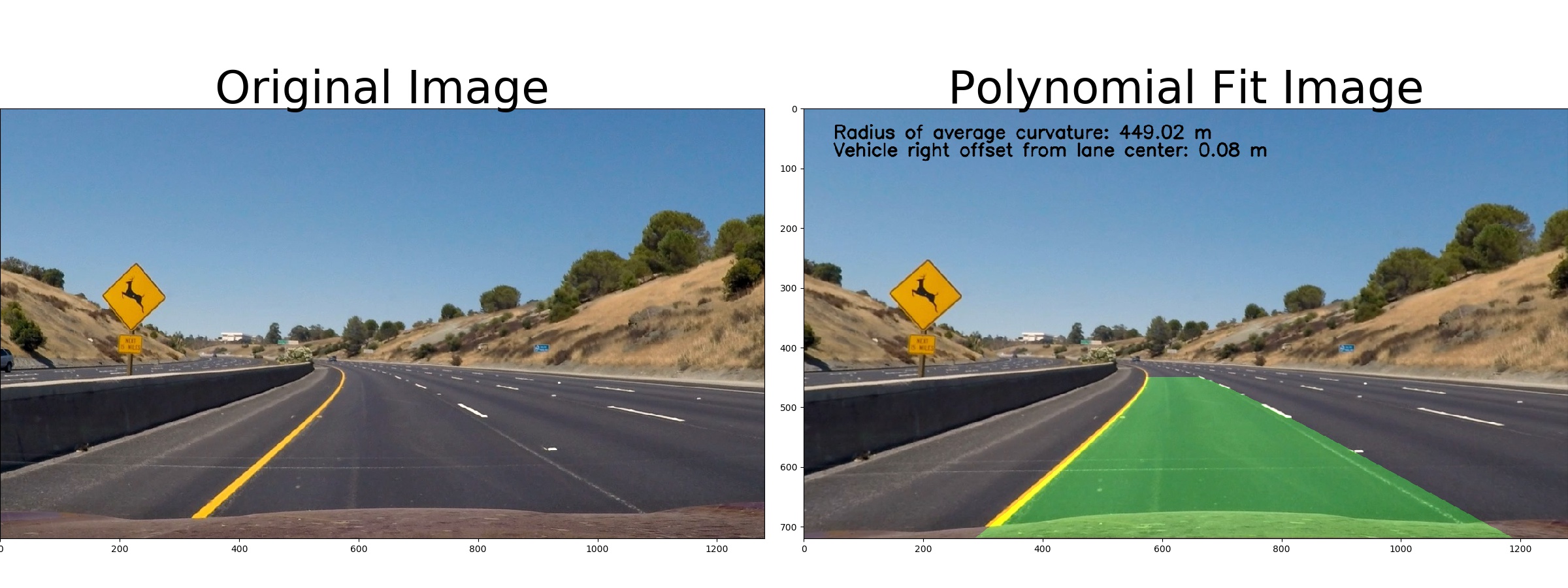
6. Provide an example image of your result plotted back down onto the road such that the lane area is identified clearly.
The code for this step is defined as final_drawing function in code lines 52-92 and process_video_image function in code lines 94-184 of Curvature_offset_process_video.py. For he smoothing fit and reseting we also define a class in Lane_class.py. you can also find them in jupyter notebook code cell 29-32.
Here I will illustrate the process of process each video image of the function process_video_image:
-
Slide windows: at the begginning, we slide windows to find left and right lanes
-
Skip Windows: once we know where the lines are you have a fit, In the next frame of video we don't need to do a blind search again, but instead you can just search in a margin around the previous line positions.(Skip the sliding windows step once we know where the lines are)
-
Smooth fit: each time we get a new high-confidence measurement, we append it to the list of recent measurements and then take an average over n past measurements to obtain the lane position we want to draw onto the image. Here we set n to 5.
-
Reset: If the lanes are not detected in a frame, we use the average values of previous n frames as corresponding values for this frame and redetect lanes in the next frame.
Here is final result for one of the test image like this:
1. Provide a link to your final video output. Your pipeline should perform reasonably well on the entire project video (wobbly lines are ok but no catastrophic failures that would cause the car to drive off the road!).
The code for this step can be found in lines 218-232 of Curvature_offset_process_video.py.
Here's a link to my video result
In future, I will try to define the source(src) and destination(dst) points automatically to make it more robust, and design more better combined threshold methods to suit more challenging situations like challenge.video.mp4 and harder_challenge_video.mp4.
1. Briefly discuss any problems / issues you faced in your implementation of this project. Where will your pipeline likely fail? What could you do to make it more robust?
If there are sunshine and shallows, it will become harder to recognize the lanes, I think I need to combine more threshold to make the recognition more robust.

