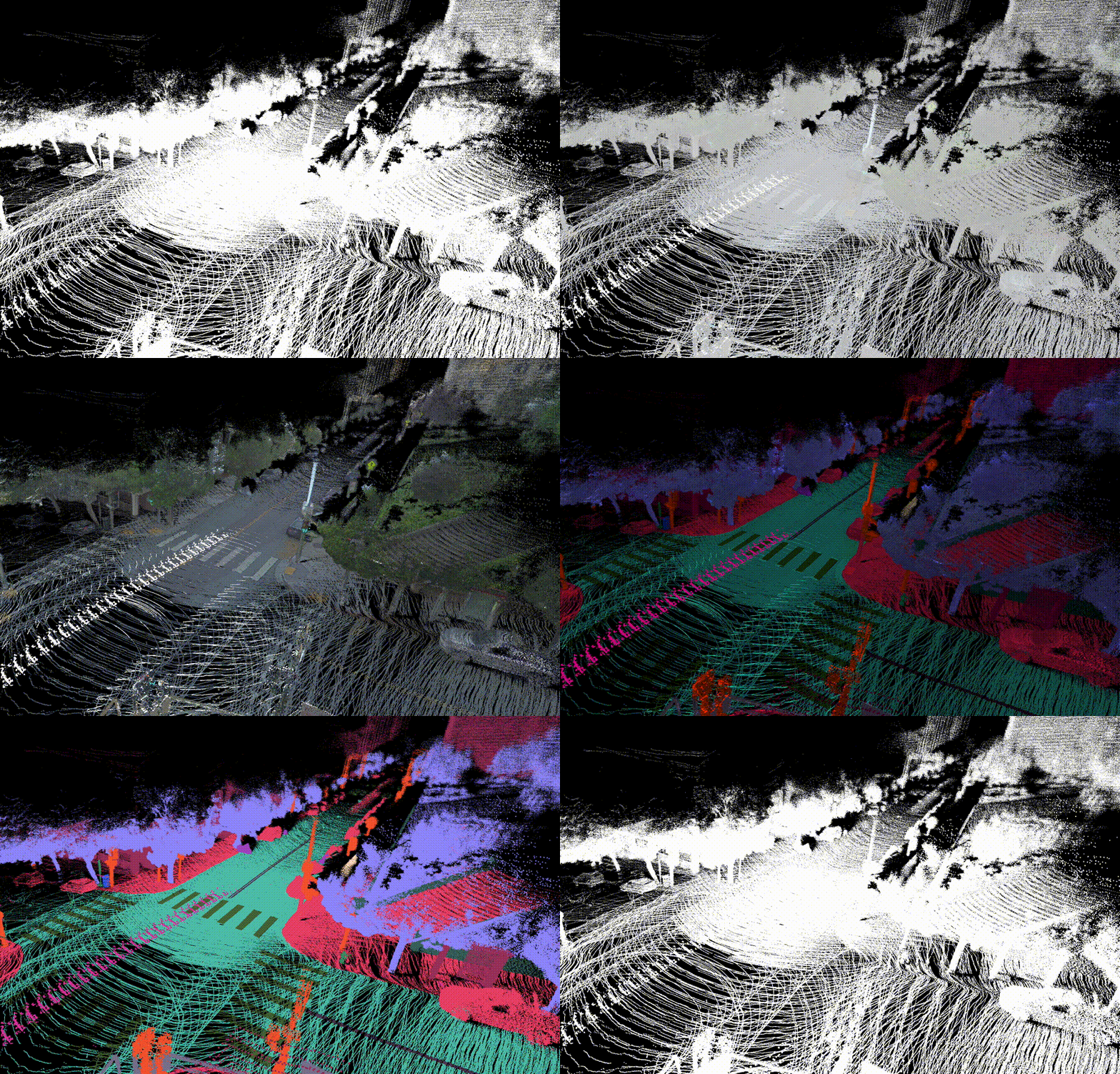
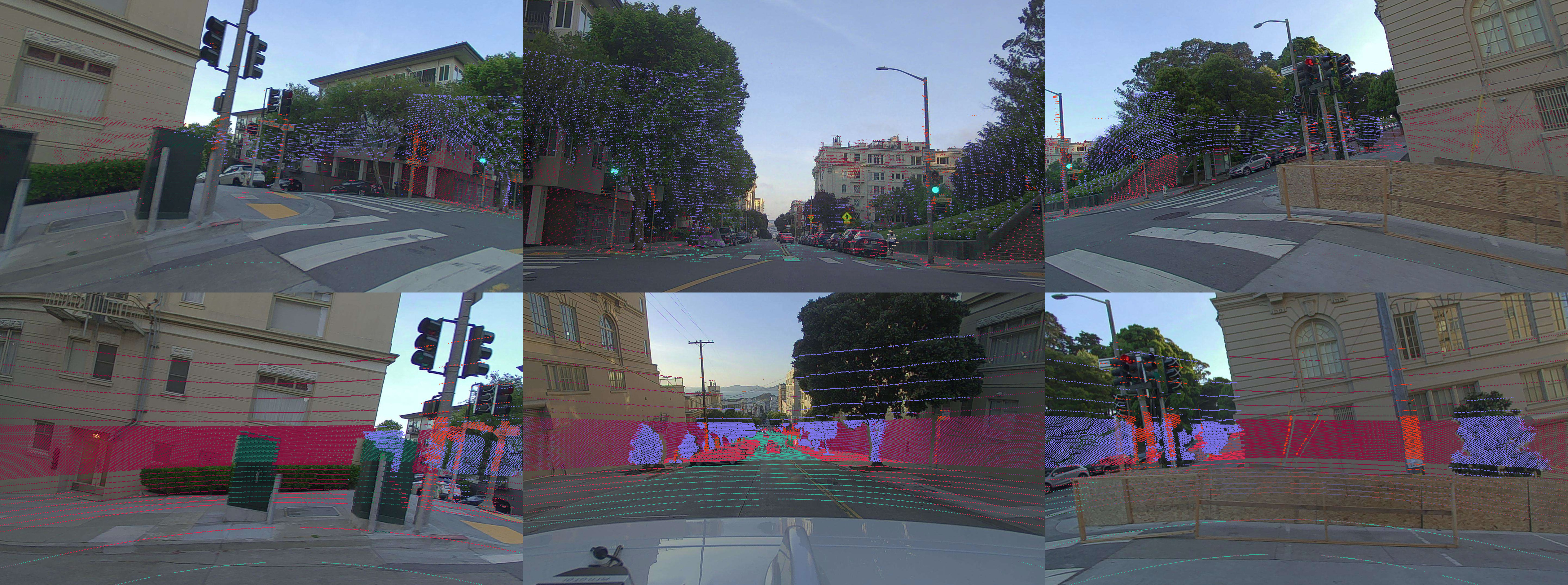
Welcome to the repository of the PandaSet Devkit.
To download the dataset, please visit the official PandaSet webpage and sign up through the form. You will then be forwarded to a page with download links to the raw data and annotations.
Unpack the archive into any directory on your hard disk. The path will be referenced in usage of pandaset-devkit later, and does not have to be in the same directory as your scripts.
.
├── LICENSE.txt
├── annotations
│   ├── cuboids
│   │   ├── 00.pkl.gz
│   │   .
│   │   .
│   │   .
│   │   └── 79.pkl.gz
│   └── semseg  // Semantic Segmentation is available for specific scenes
│       ├── 00.pkl.gz
│       .
│       .
│       .
│       ├── 79.pkl.gz
│       └── classes.json
├── camera
│   ├── back_camera
│   │   ├── 00.jpg
│   │   .
│   │   .
│   │   .
│   │   ├── 79.jpg
│   │   ├── intrinsics.json
│   │   ├── poses.json
│   │   └── timestamps.json
│   ├── front_camera
│   │   └── ...
│   ├── front_left_camera
│   │   └── ...
│   ├── front_right_camera
│   │   └── ...
│   ├── left_camera
│   │   └── ...
│   └── right_camera
│       └── ...
├── lidar
│   ├── 00.pkl.gz
│   .
│   .
│   .
│   ├── 79.pkl.gz
│   ├── poses.json
│   └── timestamps.json
└── meta
    ├── gps.json
    └── timestamps.json
- Create a Python>=3.6 environment with
pipinstalled. - Clone the repository
git clone git@github.com:scaleapi/pandaset-devkit.git cdintopandaset-devkit/python- Execute
pip install .
The pandaset-devkit is now installed in your Python>=3.6 environment and can be used.
To get familiar with the API you can point directly to the downloaded dataset.
First, we need to create a DataSet object that searches for sequences.
>>> from pandaset import DataSet
>>> dataset = DataSet('/data/pandaset')
Afterwards we can list all the sequence IDs that have been found in the data folder.
>>> print(dataset.sequences())
['002',...]
Since semantic segmentation annotations are not always available for scenes, we can filter to get only scenes that have both semantic segmentation as well as cuboid annotations.
>>> print(dataset.sequences(with_semseg=True))
['002',...]
Now, we access a specific sequence by choosing its key from the previously returned list, in this case sequence ID '002'
>>> seq002 = dataset['002']
API Reference: DataSet class
The devkit will automatically search the sequence directory for available sensor data, metadata and annotations and prepare the directory to be loaded explicitly. At this point no point clouds or images have been loaded into memory.
To execute the loading of sensor data and metadata into memory, we simply call the load() method on the sequence object. This will load all available sensor data and metadata.
>>> seq002.load()
If only certain data is required for analysis, there are more specific methods available, which can also be chained to each other.
>>> seq002.load_lidar().load_cuboids()
API Reference: Sequence class
The LiDAR point clouds are stored as pandas.DataFrames and therefore you are able to leverage their extensive API for data manipulation. This includes the simple return as a numpy.ndarray.
>>> pc0 = seq002.lidar[0]
>>> print(pc0)
                 x           y         z     i             t  d
index
0       -75.131138  -79.331690  3.511804   7.0  1.557540e+09  0
1      -112.588306 -118.666002  1.423499  31.0  1.557540e+09  0
2       -42.085902  -44.384891  0.593491   7.0  1.557540e+09  0
3       -27.329435  -28.795053 -0.403781   0.0  1.557540e+09  0
4        -6.196208   -6.621082  1.130009   3.0  1.557540e+09  0
            ...         ...       ...   ...           ... ..
166763   27.670526   17.159726  3.778677  25.0  1.557540e+09  1
166764   27.703935   17.114063  3.780626  27.0  1.557540e+09  1
166765   27.560664   16.955518  3.767948  18.0  1.557540e+09  1
166766   27.384433   16.783824  3.752670  22.0  1.557540e+09  1
166767   27.228821   16.626038  3.739154  20.0  1.557540e+09  1
[166768 rows x 6 columns]
>>> pc0_np = seq002.lidar[0].values  # Returns the first LiDAR frame in the sequence as an numpy ndarray
>>> print(pc0_np)
[[-7.51311379e+01 -7.93316897e+01  3.51180427e+00  7.00000000e+00
   1.55753996e+09  0.00000000e+00]
 [-1.12588306e+02 -1.18666002e+02  1.42349938e+00  3.10000000e+01
   1.55753996e+09  0.00000000e+00]
 [-4.20859017e+01 -4.43848908e+01  5.93490847e-01  7.00000000e+00
   1.55753996e+09  0.00000000e+00]
 ...
 [ 2.75606640e+01  1.69555183e+01  3.76794770e+00  1.80000000e+01
   1.55753996e+09  1.00000000e+00]
 [ 2.73844334e+01  1.67838237e+01  3.75266969e+00  2.20000000e+01
   1.55753996e+09  1.00000000e+00]
 [ 2.72288210e+01  1.66260378e+01  3.73915448e+00  2.00000000e+01
   1.55753996e+09  1.00000000e+00]]
The LiDAR points are stored in a world coordinate system; therefore it is not required to transform them using the vehicle's pose graph. This allows you to query all LiDAR frames in the sequence or a certain sampling rate and simply visualize them using your preferred library.
Instead of using always all of the point clouds available, it is also possible to simply slice the lidar property as one is used from python lists.
>>> pc_all = seq002.lidar[:] # Returns all LiDAR frames from the sequence
>>> pc_sampled = seq002.lidar[::2] # Returns every second LiDAR frame from the sequence
In addition to the LiDAR points, the lidar property also holds the sensor pose (lidar.poses) in world coordinate system and timestamp (lidar.timestamps) for every LiDAR frame recorded. Both objects can be sliced in the same way as the lidar property holding the point clouds.
>>> sl = slice(None, None, 5)  # Equivalent to [::5]  # Extract every fifth frame including sensor pose and timestamps
>>> lidar_obj = seq002.lidar
>>> pcs = lidar_obj[sl]
>>> poses = lidar_obj.poses[sl]
>>> timestamps = lidar_obj.timestamps[sl]
>>> print( len(pcs) == len(poses) == len(timestamps) )
True
The LiDAR point clouds include by default the points from both the mechanical 360° LiDAR and the front-facing LiDAR. To select only one of the sensors, the set_sensor method is available.
>>> pc0 = s002.lidar[0]
>>> print(pc0.shape)
(166768, 6)
>>> s002.lidar.set_sensor(0)  # set to include only mechanical 360° LiDAR
>>> pc0_sensor0 = s002.lidar[0]
>>> print(pc0_sensor0.shape)
(106169, 6)
>>> s002.lidar.set_sensor(1)  # set to include only front-facing LiDAR
>>> pc0_sensor1 = s002.lidar[0]
>>> print(pc0_sensor1.shape)
(60599, 6)
Since the applied filter operation leaves the original row index intact for each point (relevant for joining with SemanticSegmentation), one can easily test that no point was left out in filtering:
>>> import pandas as pd
>>> pc0_concat = pd.concat([pc0_sensor0, pc0_sensor1])
>>> print(pc0_concat.shape)
(166768, 6)
>>> print(pc0 == pc0_concat)
           x     y     z     i     t     d
index
0       True  True  True  True  True  True
1       True  True  True  True  True  True
2       True  True  True  True  True  True
3       True  True  True  True  True  True
4       True  True  True  True  True  True
      ...   ...   ...   ...   ...   ...
166763  True  True  True  True  True  True
166764  True  True  True  True  True  True
166765  True  True  True  True  True  True
166766  True  True  True  True  True  True
166767  True  True  True  True  True  True
[166768 rows x 6 columns]
>>> print((~(pc0 == pc0_concat)).sum())  # Counts the number of cells with `False` value, i.e., the ones where original point cloud and concatenated filtered point cloud differentiate
x    0
y    0
z    0
i    0
t    0
d    0
dtype: int64
API Reference: Lidar class
Since the recording vehicle was equipped with multiple cameras, first we need to list which cameras have been used to record the sequence.
>>> print(seq002.camera.keys())
['front_camera', 'left_camera', 'back_camera', 'right_camera', 'front_left_camera', 'front_right_camera']
The camera count and names should be equal for all sequences.
Each camera name has its recordings loaded as Pillow Image object, and can be accessed via normal list slicing. In the following example, we select the first image from the front camera and display it using the Pillow library in Python.
>>> front_camera = seq002.camera['front_camera']
>>> img0 = front_camera[0]
>>> img0.show()
Afterwards the extensive Pillow Image API can be used for image manipulation, conversion or export.
Similar to the Lidar object, each Camera object has properties that hold the camera pose (camera.poses) and timestamp (camera.timestamps) for every recorded frame, as well as the camera intrinsics (camera.intrinsics).
Again, the objects can be sliced the same way as the Camera object:
>>> sl = slice(None, None, 5)  # Equivalent to [::5]
>>> camera_obj = seq002.camera['front_camera']
>>> pcs = camera_obj[sl]
>>> poses = camera_obj.poses[sl]
>>> timestamps = camera_obj.timestamps[sl]
>>> intrinsics = camera_obj.intrinsics
API Reference: Camera class
In addition to the sensor data, the loaded dataset also contains the following meta information:
- GPS Positions
- Timestamps
These can be directly accessed through the known list slicing operations, and read in their dict format. The following example shows how to get the GPS coordinates of the vehicle on the first frame.
>>> pose0 = seq002.gps[0]
>>> print(pose0['lat'])
37.776089291519924
>>> print(pose0['long'])
-122.39931707791749
API Reference: GPS class
API Reference: Timestamps class
The LiDAR Cuboid annotations are also stored inside the sequence object as a pandas.DataFrames for each timestamp.
The position coordinates (position.x,position.y,position.z) are located at the center of a cuboid. dimensions.x is the width of the cuboid from left to right, dimensions.y is the length of the cuboid from front to back and dimensions.z is the height of the cuboid from top to bottom.
>>> cuboids0 = seq002.cuboids[0]  # Returns the cuboid annotations for the first LiDAR frame in the sequence
>>> print(cuboids0.columns)
Index(['uuid', 'label', 'yaw', 'stationary', 'camera_used', 'position.x',
       'position.y', 'position.z', 'dimensions.x', 'dimensions.y',
       'dimensions.z', 'attributes.object_motion', 'cuboids.sibling_id',
       'cuboids.sensor_id', 'attributes.rider_status',
       'attributes.pedestrian_behavior', 'attributes.pedestrian_age'],
      dtype='object')
API Reference: Cuboids class
Analogous to the cuboid annotations, the Semantic Segmentation can be accessed using the semseg property on the sequence object. The index of each Semantic Segmentation data frame corresponds to the index of each LiDAR point cloud data frame, and can be joined using the index.
>>> semseg0 = seq002.semseg[0]  # Returns the semantic segmentation for the first LiDAR frame in the sequence
>>> print(semseg0.columns)
Index(['class'], dtype='object')
>>> print(seq002.semseg.classes)
{'1': 'Smoke', '2': 'Exhaust', '3': 'Spray or rain', '4': 'Reflection', '5': 'Vegetation', '6': 'Ground', '7': 'Road', '8': 'Lane Line Marking', '9': 'Stop Line Marking', '10': 'Other Road Marking', '11': 'Sidewalk', '12': 'Driveway', '13': 'Car', '14': 'Pickup Truck', '15': 'Medium-sized Truck', '16': 'Semi-truck', '17': 'Towed Object', '18': 'Motorcycle', '19': 'Other Vehicle - Construction Vehicle', '20': 'Other Vehicle - Uncommon', '21': 'Other Vehicle - Pedicab', '22': 'Emergency Vehicle', '23': 'Bus', '24': 'Personal Mobility Device', '25': 'Motorized Scooter', '26': 'Bicycle', '27': 'Train', '28': 'Trolley', '29': 'Tram / Subway', '30': 'Pedestrian', '31': 'Pedestrian with Object', '32': 'Animals - Bird', '33': 'Animals - Other', '34': 'Pylons', '35': 'Road Barriers', '36': 'Signs', '37': 'Cones', '38': 'Construction Signs', '39': 'Temporary Construction Barriers', '40': 'Rolling Containers', '41': 'Building', '42': 'Other Static Object'}
API Reference: SemanticSegmentation class

