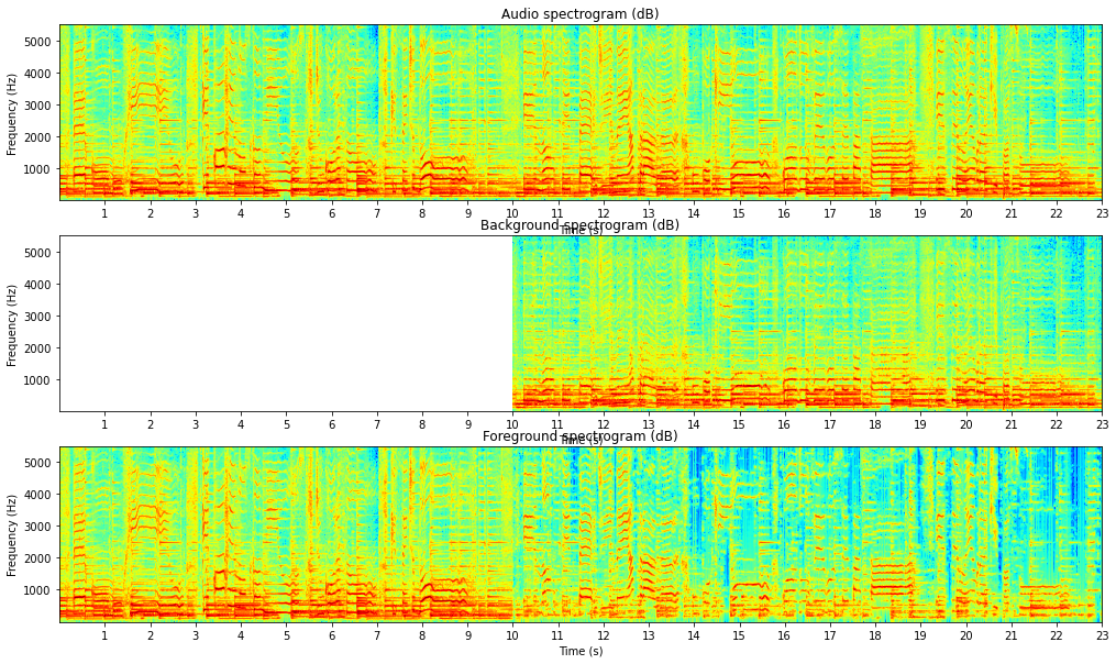
REPeating Pattern Extraction Technique (REPET) in Python for audio source separation.
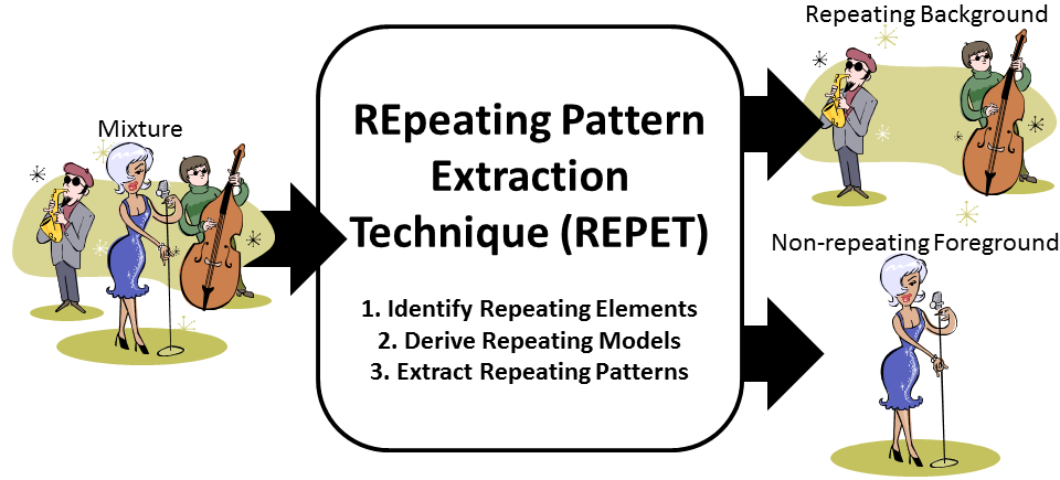
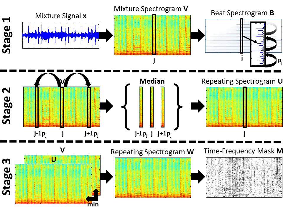
Repetition is a fundamental element in generating and perceiving structure. In audio, mixtures are often composed of structures where a repeating background signal is superimposed with a varying foreground signal (e.g., a singer overlaying varying vocals on a repeating accompaniment or a varying speech signal mixed up with a repeating background noise). On this basis, we present the REpeating Pattern Extraction Technique (REPET), a simple approach for separating the repeating background from the non-repeating foreground in an audio mixture. The basic idea is to find the repeating elements in the mixture, derive the underlying repeating models, and extract the repeating background by comparing the models to the mixture. Unlike other separation approaches, REPET does not depend on special parameterizations, does not rely on complex frameworks, and does not require external information. Because it is only based on repetition, it has the advantage of being simple, fast, blind, and therefore completely and easily automatable.
Files:
repet.py: Python module with the REPET functions.examples.ipynb: Jupyter notebook with some examples.audio_file.wav: audio file used for the examples.
See also:
- REPET-Matlab: REPET in Matlab for audio source separation.
This Python module implements a number of functions for REPET:
Simply copy the file repet.py in your working directory and you are good to go. Make sure you have Python 3, NumPy, and SciPy installed.
Functions:
original- Compute the original REPET.extended- Compute REPET extended.adaptive- Compute the adaptive REPET.sim- Compute REPET-SIM.simonline- Compute the online REPET-SIM.
Other:
wavread- Read a WAVE file (using SciPy).wavwrite- Write a WAVE file (using SciPy).specshow- Display a spectrogram in dB, seconds, and Hz.
Compute the original REPET.
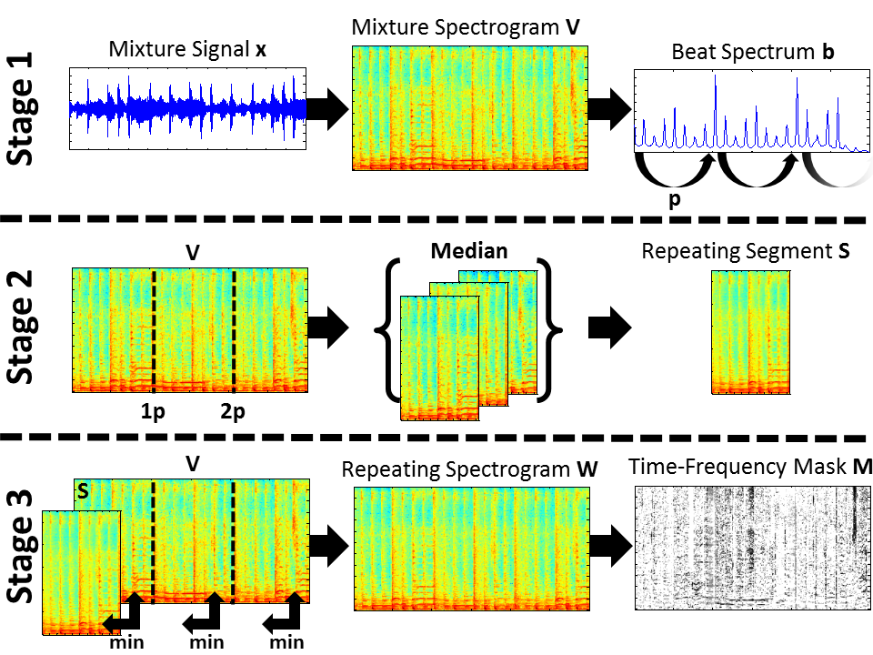
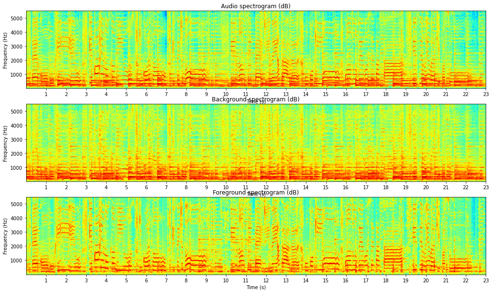
The original REPET aims at identifying and extracting the repeating patterns in an audio mixture, by estimating a period of the underlying repeating structure and modeling a segment of the periodically repeating background.
background_signal = repet.original(audio_signal, sampling_frequency)

Inputs:
    audio_signal: audio signal (number_samples, number_channels)
    sampling_frequency: sampling frequency in Hz
Output:
    background_signal: audio STFT (window_length, number_frames)
# Import the modules
import numpy as np
import scipy.signal
import repet
import matplotlib.pyplot as plt

# Read the audio signal (normalized) with its sampling frequency in Hz
audio_signal, sampling_frequency = repet.wavread("audio_file.wav")

# Estimate the background signal, and the foreground signal
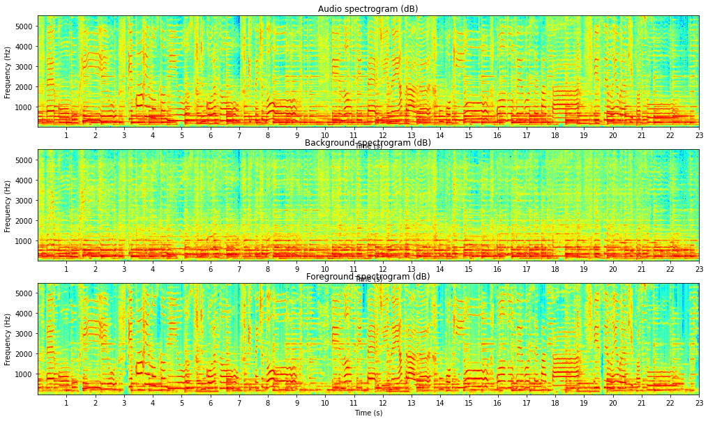
background_signal = repet.original(audio_signal, sampling_frequency)
foreground_signal = audio_signal-background_signal

# Write the background and foreground signals
repet.wavwrite(background_signal, sampling_frequency, "background_signal.wav")
repet.wavwrite(foreground_signal, sampling_frequency, "foreground_signal.wav")

# Compute the mixture, background, and foreground spectrograms
window_length = pow(2, int(np.ceil(np.log2(0.04*sampling_frequency))))
window_function = scipy.signal.hamming(window_length, sym=False)
step_length = int(window_length/2)
number_frequencies = int(window_length/2)+1
audio_spectrogram = abs(repet._stft(np.mean(audio_signal, axis=1), window_function, step_length)[0:number_frequencies, :])
background_spectrogram = abs(repet._stft(np.mean(background_signal, axis=1), window_function, step_length)[0:number_frequencies, :])
foreground_spectrogram = abs(repet._stft(np.mean(foreground_signal, axis=1), window_function, step_length)[0:number_frequencies, :])

# Display the mixture, background, and foreground spectrograms in dB, seconds, and Hz
time_duration = len(audio_signal)/sampling_frequency
maximum_frequency = sampling_frequency/8
xtick_step = 1
ytick_step = 1000
plt.figure(figsize=(17, 10))
plt.subplot(3,1,1)
repet.specshow(audio_spectrogram[0:int(window_length/8), :], time_duration, maximum_frequency, xtick_step, ytick_step)
plt.title("Audio spectrogram (dB)")
plt.subplot(3,1,2)
repet.specshow(background_spectrogram[0:int(window_length/8), :], time_duration, maximum_frequency, xtick_step, ytick_step)
plt.title("Background spectrogram (dB)")
plt.subplot(3,1,3)
repet.specshow(foreground_spectrogram[0:int(window_length/8), :], time_duration, maximum_frequency, xtick_step, ytick_step)
plt.title("Foreground spectrogram (dB)")
plt.show()
Compute REPET extended.
The original REPET can be easily extended to handle varying repeating structures, by simply applying the method along time, on individual segments or via a sliding window.
background_signal = repet.extended(audio_signal, sampling_frequency)

Inputs:
    audio_signal: audio signal (number_samples, number_channels)
    sampling_frequency: sampling frequency in Hz
Output:
    background_signal: audio STFT (window_length, number_frames)
# Import the modules
import numpy as np
import scipy.signal
import repet
import matplotlib.pyplot as plt

# Read the audio signal (normalized) with its sampling frequency in Hz
audio_signal, sampling_frequency = repet.wavread("audio_file.wav")

# Estimate the background signal, and the foreground signal
background_signal = repet.extended(audio_signal, sampling_frequency)
foreground_signal = audio_signal-background_signal

# Write the background and foreground signals
repet.wavwrite(background_signal, sampling_frequency, "background_signal.wav")
repet.wavwrite(foreground_signal, sampling_frequency, "foreground_signal.wav")

# Compute the mixture, background, and foreground spectrograms
window_length = pow(2, int(np.ceil(np.log2(0.04*sampling_frequency))))
window_function = scipy.signal.hamming(window_length, sym=False)
step_length = int(window_length/2)
number_frequencies = int(window_length/2)+1
audio_spectrogram = abs(repet._stft(np.mean(audio_signal, axis=1), window_function, step_length)[0:number_frequencies, :])
background_spectrogram = abs(repet._stft(np.mean(background_signal, axis=1), window_function, step_length)[0:number_frequencies, :])
foreground_spectrogram = abs(repet._stft(np.mean(foreground_signal, axis=1), window_function, step_length)[0:number_frequencies, :])

# Display the mixture, background, and foreground spectrograms in dB, seconds, and Hz
time_duration = len(audio_signal)/sampling_frequency
maximum_frequency = sampling_frequency/8
xtick_step = 1
ytick_step = 1000
plt.figure(figsize=(17, 10))
plt.subplot(3,1,1)
repet.specshow(audio_spectrogram[0:int(window_length/8), :], time_duration, maximum_frequency, xtick_step, ytick_step)
plt.title("Audio spectrogram (dB)")
plt.subplot(3,1,2)
repet.specshow(background_spectrogram[0:int(window_length/8), :], time_duration, maximum_frequency, xtick_step, ytick_step)
plt.title("Background spectrogram (dB)")
plt.subplot(3,1,3)
repet.specshow(foreground_spectrogram[0:int(window_length/8), :], time_duration, maximum_frequency, xtick_step, ytick_step)
plt.title("Foreground spectrogram (dB)")
plt.show()
Compute the adaptive REPET.
The original REPET works well when the repeating background is relatively stable (e.g., a verse or the chorus in a song); however, the repeating background can also vary over time (e.g., a verse followed by the chorus in the song). The adaptive REPET is an extension of the original REPET that can handle varying repeating structures, by estimating the time-varying repeating periods and extracting the repeating background locally, without the need for segmentation or windowing.
background_signal = repet.adaptive(audio_signal, sampling_frequency)

Inputs:
    audio_signal: audio signal (number_samples, number_channels)
    sampling_frequency: sampling frequency in Hz
Output:
    background_signal: audio STFT (window_length, number_frames)
# Import the modules
import numpy as np
import scipy.signal
import repet
import matplotlib.pyplot as plt

# Read the audio signal (normalized) with its sampling frequency in Hz
audio_signal, sampling_frequency = repet.wavread("audio_file.wav")

# Estimate the background signal, and the foreground signal
background_signal = repet.adaptive(audio_signal, sampling_frequency)
foreground_signal = audio_signal-background_signal

# Write the background and foreground signals
repet.wavwrite(background_signal, sampling_frequency, "background_signal.wav")
repet.wavwrite(foreground_signal, sampling_frequency, "foreground_signal.wav")

# Compute the mixture, background, and foreground spectrograms
window_length = pow(2, int(np.ceil(np.log2(0.04*sampling_frequency))))
window_function = scipy.signal.hamming(window_length, sym=False)
step_length = int(window_length/2)
number_frequencies = int(window_length/2)+1
audio_spectrogram = abs(repet._stft(np.mean(audio_signal, axis=1), window_function, step_length)[0:number_frequencies, :])
background_spectrogram = abs(repet._stft(np.mean(background_signal, axis=1), window_function, step_length)[0:number_frequencies, :])
foreground_spectrogram = abs(repet._stft(np.mean(foreground_signal, axis=1), window_function, step_length)[0:number_frequencies, :])

# Display the mixture, background, and foreground spectrograms in dB, seconds, and Hz
time_duration = len(audio_signal)/sampling_frequency
maximum_frequency = sampling_frequency/8
xtick_step = 1
ytick_step = 1000
plt.figure(figsize=(17, 10))
plt.subplot(3,1,1)
repet.specshow(audio_spectrogram[0:int(window_length/8), :], time_duration, maximum_frequency, xtick_step, ytick_step)
plt.title("Audio spectrogram (dB)")
plt.subplot(3,1,2)
repet.specshow(background_spectrogram[0:int(window_length/8), :], time_duration, maximum_frequency, xtick_step, ytick_step)
plt.title("Background spectrogram (dB)")
plt.subplot(3,1,3)
repet.specshow(foreground_spectrogram[0:int(window_length/8), :], time_duration, maximum_frequency, xtick_step, ytick_step)
plt.title("Foreground spectrogram (dB)")
plt.show()
Compute REPET-SIM.
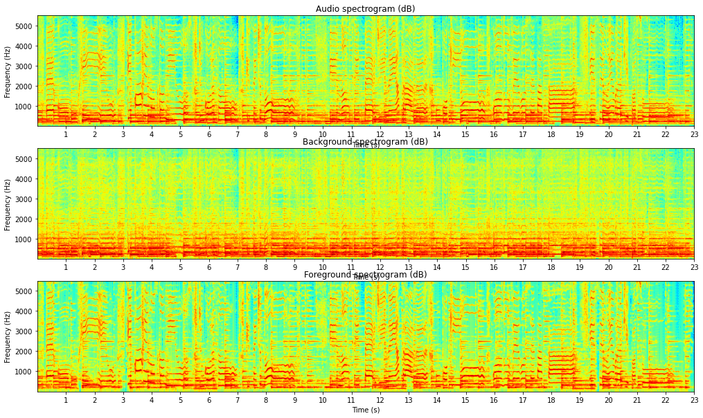
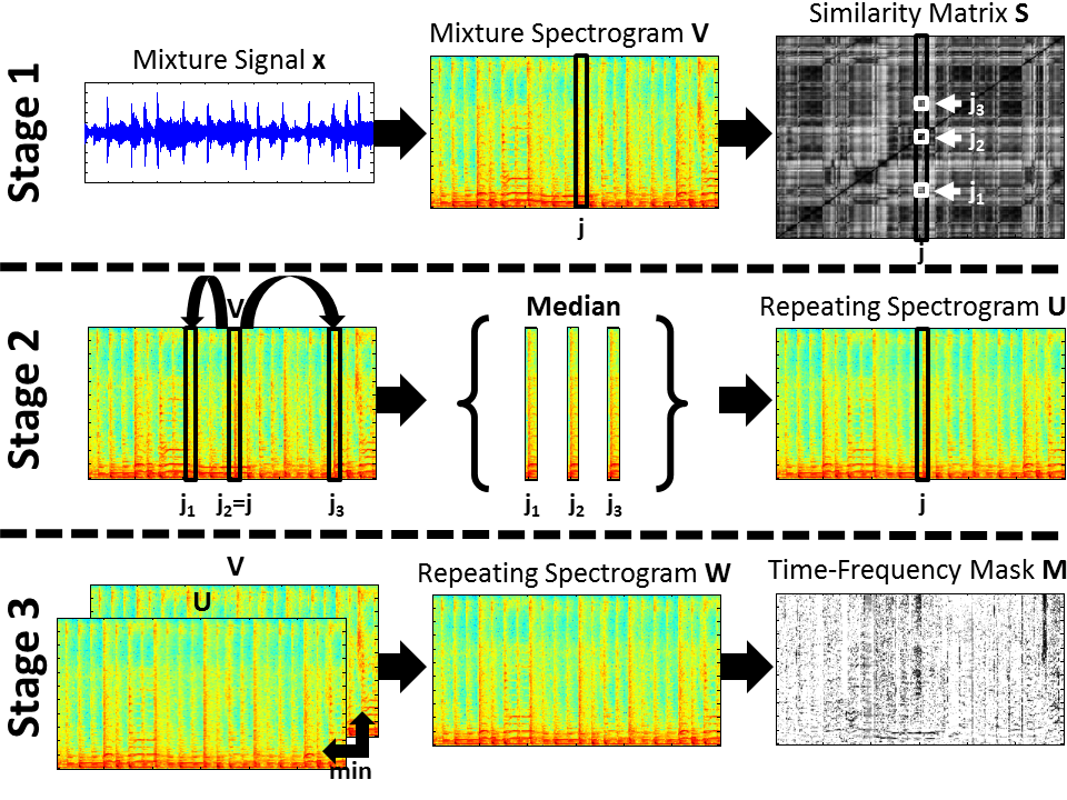
The REPET methods work well when the repeating background has periodically repeating patterns (e.g., jackhammer noise); however, the repeating patterns can also happen intermittently or without a global or local periodicity (e.g., frogs by a pond). REPET-SIM is a generalization of REPET that can also handle non-periodically repeating structures, by using a similarity matrix to identify the repeating elements.
background_signal = repet.sim(audio_signal, sampling_frequency)

Inputs:
    audio_signal: audio signal (number_samples, number_channels)
    sampling_frequency: sampling frequency in Hz
Output:
    background_signal: audio STFT (window_length, number_frames)
# Import the modules
import numpy as np
import scipy.signal
import repet
import matplotlib.pyplot as plt

# Read the audio signal (normalized) with its sampling frequency in Hz
audio_signal, sampling_frequency = repet.wavread("audio_file.wav")

# Estimate the background signal, and the foreground signal
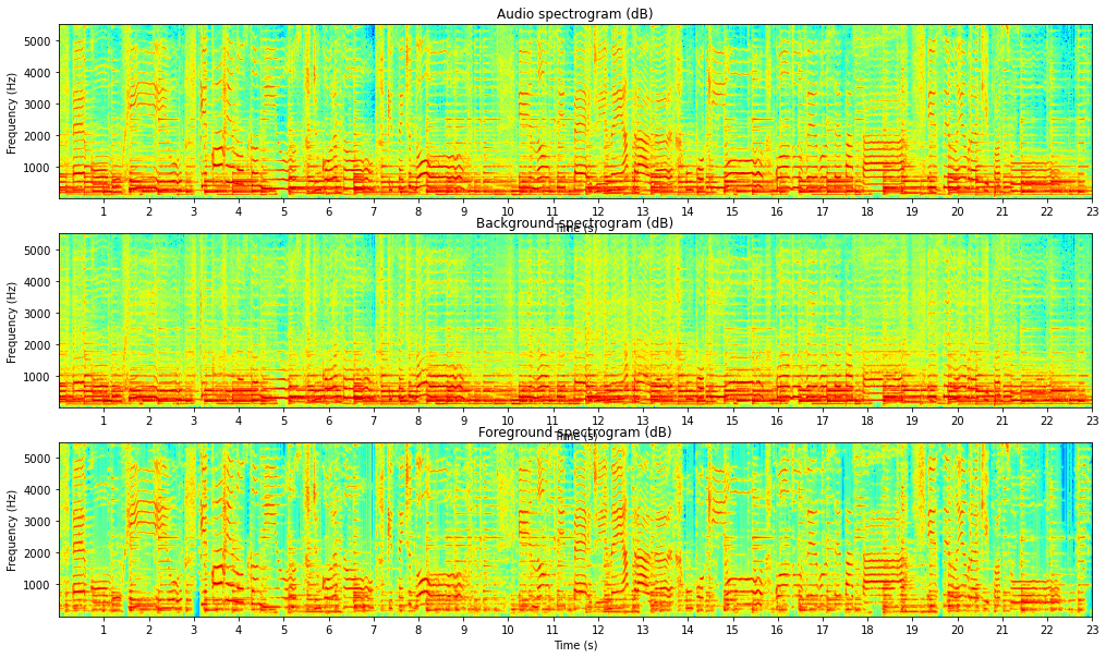
background_signal = repet.sim(audio_signal, sampling_frequency)
foreground_signal = audio_signal-background_signal

# Write the background and foreground signals
repet.wavwrite(background_signal, sampling_frequency, "background_signal.wav")
repet.wavwrite(foreground_signal, sampling_frequency, "foreground_signal.wav")

# Compute the mixture, background, and foreground spectrograms
window_length = pow(2, int(np.ceil(np.log2(0.04*sampling_frequency))))
window_function = scipy.signal.hamming(window_length, sym=False)
step_length = int(window_length/2)
number_frequencies = int(window_length/2)+1
audio_spectrogram = abs(repet._stft(np.mean(audio_signal, axis=1), window_function, step_length)[0:number_frequencies, :])
background_spectrogram = abs(repet._stft(np.mean(background_signal, axis=1), window_function, step_length)[0:number_frequencies, :])
foreground_spectrogram = abs(repet._stft(np.mean(foreground_signal, axis=1), window_function, step_length)[0:number_frequencies, :])

# Display the mixture, background, and foreground spectrograms in dB, seconds, and Hz
time_duration = len(audio_signal)/sampling_frequency
maximum_frequency = sampling_frequency/8
xtick_step = 1
ytick_step = 1000
plt.figure(figsize=(17, 10))
plt.subplot(3,1,1)
repet.specshow(audio_spectrogram[0:int(window_length/8), :], time_duration, maximum_frequency, xtick_step, ytick_step)
plt.title("Audio spectrogram (dB)")
plt.subplot(3,1,2)
repet.specshow(background_spectrogram[0:int(window_length/8), :], time_duration, maximum_frequency, xtick_step, ytick_step)
plt.title("Background spectrogram (dB)")
plt.subplot(3,1,3)
repet.specshow(foreground_spectrogram[0:int(window_length/8), :], time_duration, maximum_frequency, xtick_step, ytick_step)
plt.title("Foreground spectrogram (dB)")
plt.show()
Compute the online REPET-SIM.
REPET-SIM can be easily implemented online to handle real-time computing, particularly for real-time speech enhancement. The online REPET-SIM simply processes the time frames of the mixture one after the other given a buffer that temporally stores past frames.
background_signal = repet.simonline(audio_signal, sampling_frequency)

Inputs:
    audio_signal: audio signal (number_samples, number_channels)
    sampling_frequency: sampling frequency in Hz
Output:
    background_signal: audio STFT (window_length, number_frames)
# Import the modules
import numpy as np
import scipy.signal
import repet
import matplotlib.pyplot as plt

# Read the audio signal (normalized) with its sampling frequency in Hz
audio_signal, sampling_frequency = repet.wavread("audio_file.wav")

# Estimate the background signal, and the foreground signal
background_signal = repet.simonline(audio_signal, sampling_frequency)
foreground_signal = audio_signal-background_signal

# Write the background and foreground signals
repet.wavwrite(background_signal, sampling_frequency, "background_signal.wav")
repet.wavwrite(foreground_signal, sampling_frequency, "foreground_signal.wav")

# Compute the mixture, background, and foreground spectrograms
window_length = pow(2, int(np.ceil(np.log2(0.04*sampling_frequency))))
window_function = scipy.signal.hamming(window_length, sym=False)
step_length = int(window_length/2)
number_frequencies = int(window_length/2)+1
audio_spectrogram = abs(repet._stft(np.mean(audio_signal, axis=1), window_function, step_length)[0:number_frequencies, :])
background_spectrogram = abs(repet._stft(np.mean(background_signal, axis=1), window_function, step_length)[0:number_frequencies, :])
foreground_spectrogram = abs(repet._stft(np.mean(foreground_signal, axis=1), window_function, step_length)[0:number_frequencies, :])

# Display the mixture, background, and foreground spectrograms in dB, seconds, and Hz
time_duration = len(audio_signal)/sampling_frequency
maximum_frequency = sampling_frequency/8
xtick_step = 1
ytick_step = 1000
plt.figure(figsize=(17, 10))
plt.subplot(3,1,1)
repet.specshow(audio_spectrogram[0:int(window_length/8), :], time_duration, maximum_frequency, xtick_step, ytick_step)
plt.title("Audio spectrogram (dB)")
plt.subplot(3,1,2)
repet.specshow(background_spectrogram[0:int(window_length/8), :], time_duration, maximum_frequency, xtick_step, ytick_step)
plt.title("Background spectrogram (dB)")
plt.subplot(3,1,3)
repet.specshow(foreground_spectrogram[0:int(window_length/8), :], time_duration, maximum_frequency, xtick_step, ytick_step)
plt.title("Foreground spectrogram (dB)")
plt.show()
23 second audio excerpt from the song Que Pena Tanto Faz performed by Tamy.
-
Bryan Pardo, Zafar Rafii, and Zhiyao Duan. "Audio Source Separation in a Musical Context," Handbook of Systematic Musicology, Springer, Berlin, Heidelberg, 2018. [article]
-
Zafar Rafii, Antoine Liutkus, and Bryan Pardo. "REPET for Background/Foreground Separation in Audio," Blind Source Separation, Springer, Berlin, Heidelberg, 2014. [article]
-
Zafar Rafii and Bryan Pardo. "Online REPET-SIM for Real-time Speech Enhancement," 38th IEEE International Conference on Acoustics, Speech and Signal Processing, Vancouver, BC, Canada, May 26-31, 2013. [article][poster]
-
Zafar Rafii and Bryan Pardo. "Audio Separation System and Method," 13612413, March 2013. [URL]
-
Zafar Rafii and Bryan Pardo. "REpeating Pattern Extraction Technique (REPET): A Simple Method for Music/Voice Separation," IEEE Transactions on Audio, Speech, and Language Processing, vol. 21, no. 1, January 2013. [article]
-
Zafar Rafii and Bryan Pardo. "Music/Voice Separation using the Similarity Matrix," 13th International Society on Music Information Retrieval, Porto, Portugal, October 8-12, 2012. [article][slides]
-
Antoine Liutkus, Zafar Rafii, Roland Badeau, Bryan Pardo, and Gaël Richard. "Adaptive Filtering for Music/Voice Separation Exploiting the Repeating Musical Structure," 37th IEEE International Conference on Acoustics, Speech and Signal Processing, Kyoto, Japan, March 25-30, 2012. [article][slides]
-
Zafar Rafii and Bryan Pardo. "A Simple Music/Voice Separation Method based on the Extraction of the Repeating Musical Structure," 36th IEEE International Conference on Acoustics, Speech and Signal Processing, Prague, Czech Republic, May 22-27, 2011. [article][poster]
- Zafar Rafii
- http://zafarrafii.com/
- CV
- GitHub
- Google Scholar
