This guide provides an overview of how to get started with the SNPio library. It covers the basic steps to read, manipulate, and analyze genotype data using the VCFReader, PhylipReader, StructureReader, and NRemover2 classes. SNPio is designed to simplify the process of handling genotype data and preparing it for downstream analysis, such as population genetics, phylogenetics, and machine learning. The library supports various file formats, including VCF, PHYLIP, and STRUCTURE, and provides tools for filtering, encoding, and visualizing genotype data. This guide will help you get up and running with SNPio quickly and efficiently.
VCFReader, PhylipReader, and StructureReader classes are used to
read genotype data from VCF, PHYLIP, and STRUCTURE files, respectively.
These classes load the data into a GenotypeData object that has
various useful methods and properties.
The NRemover2 class is used to filter genotype data based on various
criteria, such as missing data, minor allele count, minor allele
frequency, and more. The GenotypeEncoder class is used to encode
genotype data into different formats, such as one-hot encoding, integer
encoding, and 0-1-2 encoding, for downstream analysis and machine
learning tasks.
Below is a step-by-step guide to using SNPio to read, filter, and encode genotype data for analysis.
Before using SNPio, ensure it is installed in your Python environment. You can install it using pip. In the project root directory (the directory containing setup.py), type the following command into your terminal:
pip install snpioWe recommend using a virtual environment to manage your Python packages. If you do not have a virtual environment set up, you can create one using the following commands:
python3 -m venv snpio_env
source snpio_env/bin/activate
This will create a virtual environment named snpio_env and activate
it. You can then install SNPio in this virtual environment using the pip
command mentioned above.
Note:
SNPio does not support Windows operating systems at the moment. We recommend using a Unix-based operating system such as Linux or macOS.
Note:
We aim to support anaconda environments in the future. For now, we
recommend using a virtual environment with pip to install SNPio.
To start using SNPio, import the necessary modules:
# Import the necessary modules
from snpio import (
    NRemover2,
    VCFReader,
    PhylipReader,
    StructureReader,
    Plotting,
    GenotypeEncoder,
)
Example usage:
# Define input filenames
vcf = "snpio/example_data/vcf_files/phylogen_subset14K_sorted.vcf.gz"
popmap = "snpio/example_data/popmaps/phylogen_nomx.popmap"

# Load the genotype data from a VCF file
gd = VCFReader(
    filename=vcf,
    popmapfile=popmap,
    force_popmap=True,
    verbose=True,
    plot_format="png",
    plot_fontsize=20,
    plot_dpi=300,
    despine=True,
    prefix="snpio_example"
)
You can also include or exclude any populations from the analysis by
using the include_pops and exclude_pops parameters in the reader
classes. For example:
# Only include the populations "ON", "DS", "EA", "GU", and "TT"
# Exclude the populations "MX", "YU", and "CH"
gd = VCFReader(
    filename=vcf,
    popmapfile=popmap,
    force_popmap=True,
    verbose=True,
    plot_format="png",
    plot_fontsize=20,
    plot_dpi=300,
    despine=True,
    prefix="snpio_example",
    include_pops=["ON", "DS", "EA", "GU"],
    exclude_pops=["MX", "YU", "CH"],
)
The include_pops and exclude_pops parameters are optional and can be
used to filter the populations included in the analysis. If both
parameters are provided, the populations in include_pops will be
included, and the populations in exclude_pops will be excluded.
However, populations cannot overlap between lists.
-
The
VCFReader,PhylipReader,StructureReader,NRemover2, andGenotypeEncoderclasses treat the following characters as missing data:- "N"
- "."
- "?"
- "-"
-
The
VCFReaderclass can read both uncompressed and compressed VCF files (gzipped). If your input file is in PHYLIP or STRUCTURE format, it will be forced to be biallelic. To handle more than two alleles per site, use the VCF format.
To use VCFReader, PhylipReader, or StructureReader, you can
optionally use a population map (popmap) file. This is a simple
two-column, whitespace-delimited or comma-delimited file with SampleIDs
in the first column and the corresponding PopulationIDs in the second
column. It can optionally contain a header line, with the first column
labeled "SampleID" and the second column labeled "PopulationID"
(case-insensitive). The population IDs can be any string, such as
"Population1", "Population2", etc, or an integer. SampleIDs must match
the sample names in the alignment file.
For example:
Sample1,Population1
Sample2,Population1
Sample3,Population2
Sample4,Population2
Or, with a header:
SampleID,PopulationID
Sample1,Population1
Sample2,Population1
Sample3,Population2
Sample4,Population2
The population map file is used to assign samples to populations and is useful for filtering and visualizing genotype data by population. If you do not provide a population map file, the samples will be treated as a single population.
The population map file can be provided as an argument to the reader classes. For example:
vcf = "snpio/example_data/vcf_files/phylogen_subset14K_sorted.vcf.gz"
popmap = "snpio/example_data/popmaps/phylogen_nomx.popmap"

gd = VCFReader(
    filename=vcf,
    popmapfile=popmap,
    force_popmap=True,
    verbose=True,
    plot_format="png",
    plot_fontsize=20,
    plot_dpi=300,
    despine=True,
    prefix="snpio_example"
)
Note:
The force_popmap parameter in the reader classes is used to force the
population map file to align with the samples in the alignment without
an error. If set to False, the population map file must match the
samples in the alignment exactly, and if they do not match, an error
will be raised. If set to True, the population map file will be forced
to align with the samples in the alignment by removing extra samples.
This parameter is set to False by default.
The verbose parameter in the reader classes is used to print
additional information about the genotype data and filtering steps.
The plot_format, plot_fontsize, plot_dpi, and despine parameters
in the reader classes are used to customize the output plots generated
by the reader classes. See API documentation for more details.
SNPio provides readers for different file formats. Here are examples of how to read genotype data from various file formats:
vcf = "snpio/example_data/vcf_files/phylogen_subset14K_sorted.vcf.gz"
popmap = "snpio/example_data/popmaps/phylogen_nomx.popmap"

gd = VCFReader(
    filename=vcf,
    popmapfile=popmap,
    force_popmap=True,
    verbose=True,
    plot_format="png",
    plot_fontsize=20,
    plot_dpi=300,
    despine=True,
    prefix="snpio_example",
    exclude_pops=["MX", "YU", "CH"],
    include_pops=["ON", "DS", "EA", "GU", "TT"],
)
This will read the genotype data from a VCF file and apply the population map if provided.
If you would like to read a Phylip file, you can use the PhylipReader
class:
phylip = "snpio/example_data/phylip_files/phylogen_subset14K.phy"
popmap = "snpio/example_data/popmaps/phylogen_nomx.popmap"

gd = PhylipReader(
    filename=phylip,
    popmapfile=popmap,
    force_popmap=True,
    verbose=True,
    plot_format="png",
    plot_fontsize=20,
    plot_dpi=300,
    despine=True,
    prefix="snpio_example",
    exclude_pops=["MX", "YU", "CH"],
    include_pops=["ON", "DS", "EA", "GU", "TT"],
)If you would like to read in a Structure file, you can use the
StructureReader class. For example:
structure = "snpio/example_data/structure_files/phylogen_subset14K.str"
popmap = "snpio/example_data/popmaps/phylogen_nomx.popmap"

gd = StructureReader(
    filename=structure,
    popmapfile=popmap,
    force_popmap=True,
    verbose=True,
    plot_format="png",
    plot_fontsize=20,
    plot_dpi=300,
    despine=True,
    prefix="snpio_example",
    exclude_pops=["MX", "YU", "CH"],
    include_pops=["ON", "DS", "EA", "GU", "TT"],
)
Note:
The StructureReader class will automatically detect the format of the
STRUCTURE file. It can be in one-line or two-line format (see STRUCTURE
documentation), and can optionally contain population information in the
file as the second tab-delimited column. If the population information
is not provided in the STRUCTURE file, you can provide a population map
file to assign samples to populations.
VCFReader(filename, popmapfile, force_popmap, ...): Reads and writes
genotype data from/ to a VCF file and applies a population map if
provided.
write_vcf(output_file): Writes the filtered or modified genotype data
back to a VCF file (for all three readers).
PhylipReader(filename, popmapfile, force_popmap, ...): Reads and
writes genotype data from/ to a PHYLIP file and applies a population
map.
write_phylip(output_file): Writes the filtered or modified genotype
data back to a PHYLIP file (for PhylipReader).
StructureReader(filename, popmapfile, force_popmap, ...): Reads and
writes genotype data from/ to a STRUCTURE file and applies a population
map.
write_structure(output_file): Writes the filtered or modified genotype
data back to a STRUCTURE file (for StructureReader).
Note:
The write_vcf, write_phylip, and write_structure methods are used
to write the filtered or modified genotype data back to a VCF, PHYLIP,
or STRUCTURE file, respectively. These methods can also be used to
convert between file VCF, PHYLIP, and STRUCTURE formats.
The GenotypeData along with the Plotting classes have several useful
methods for working with genotype data:
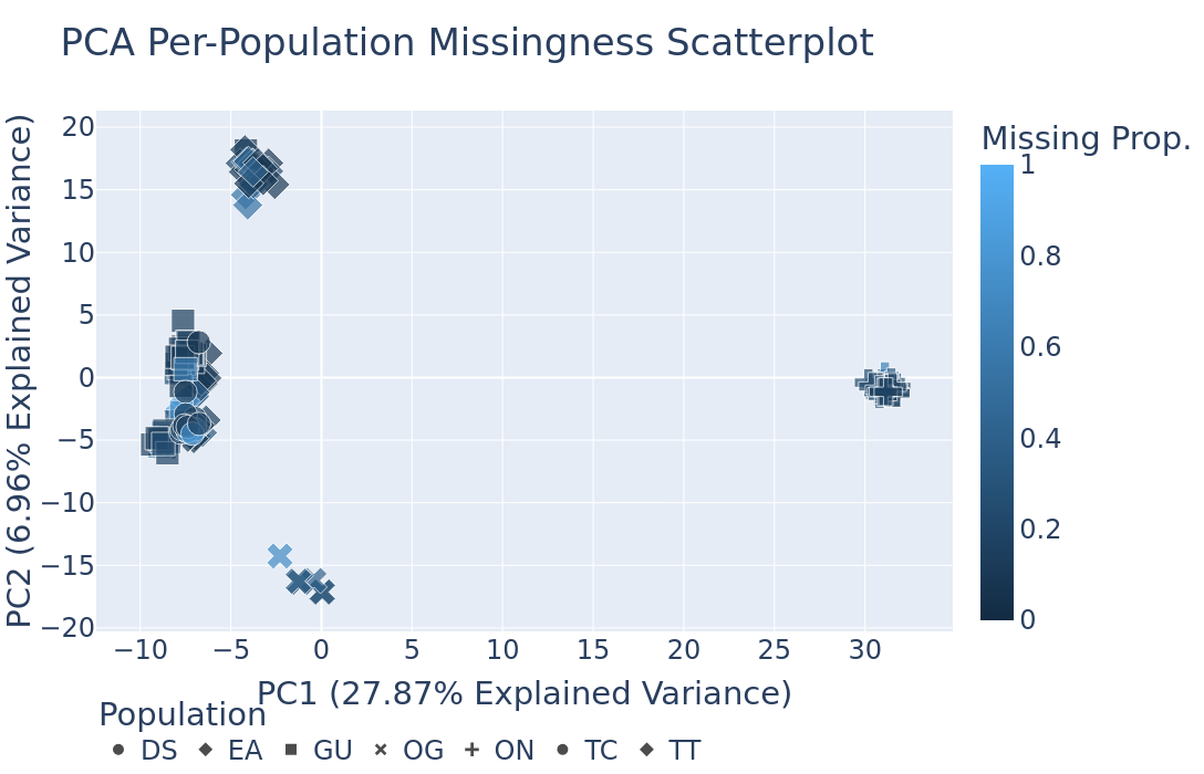
Plotting.run_pca(): Runs principal component analysis (PCA) on the genotype data and plots the results. The PCA plot can help visualize the genetic structure of the populations in the dataset, with each point representing an individual. Individuals are colored by missing data proportion, and populations are represented by different shapes. A 2-dimensional PCA plot is generated by default, but you can specify three PCA axes as well. For example:
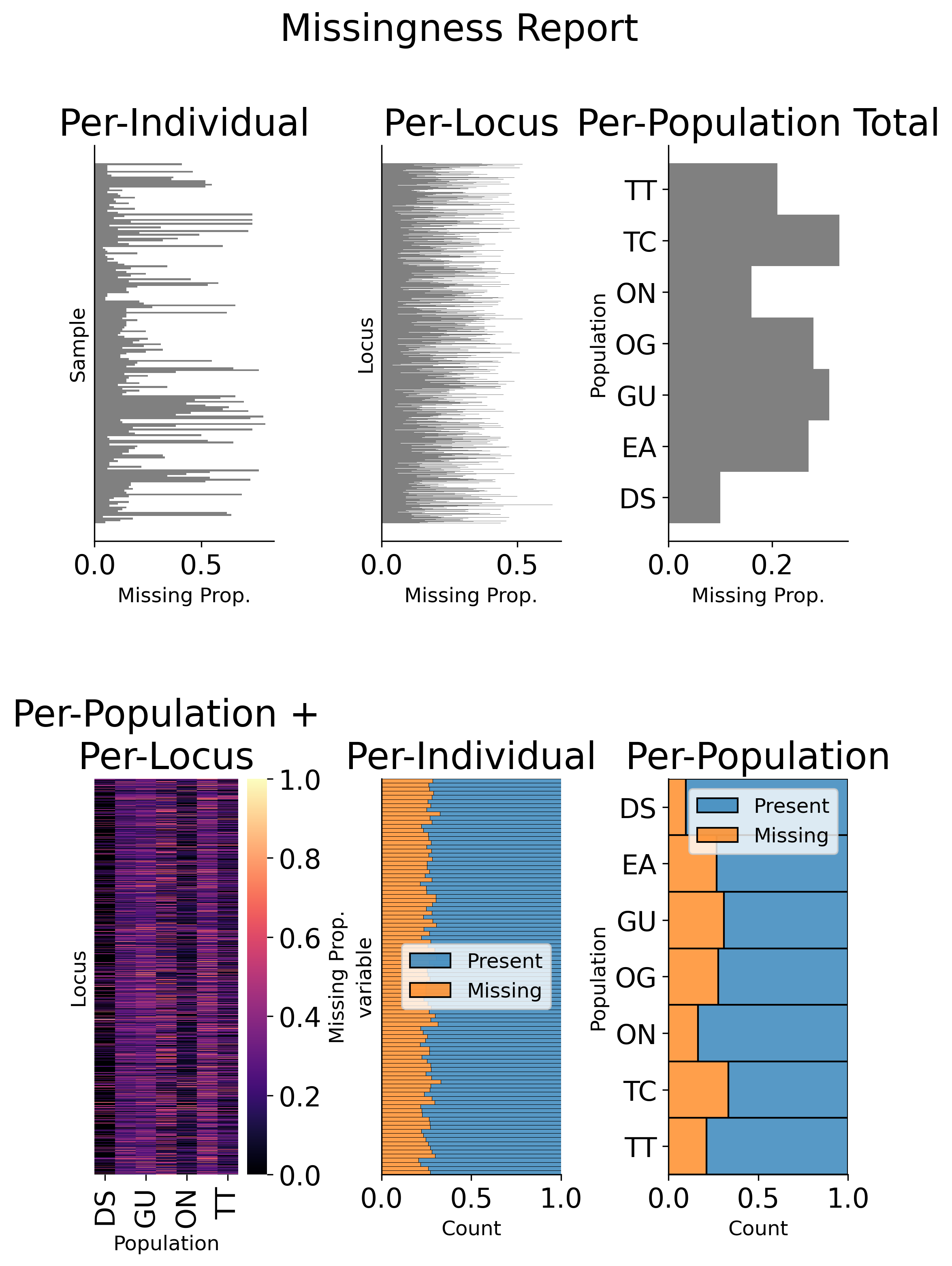
GenotypeData.missingness_reports(): Generates missing data reports and plots for the dataset. The reports include the proportion of missing data per individual, per locus, and per population. These reports can help you identify samples, loci, or populations with high levels of missing data. For example:
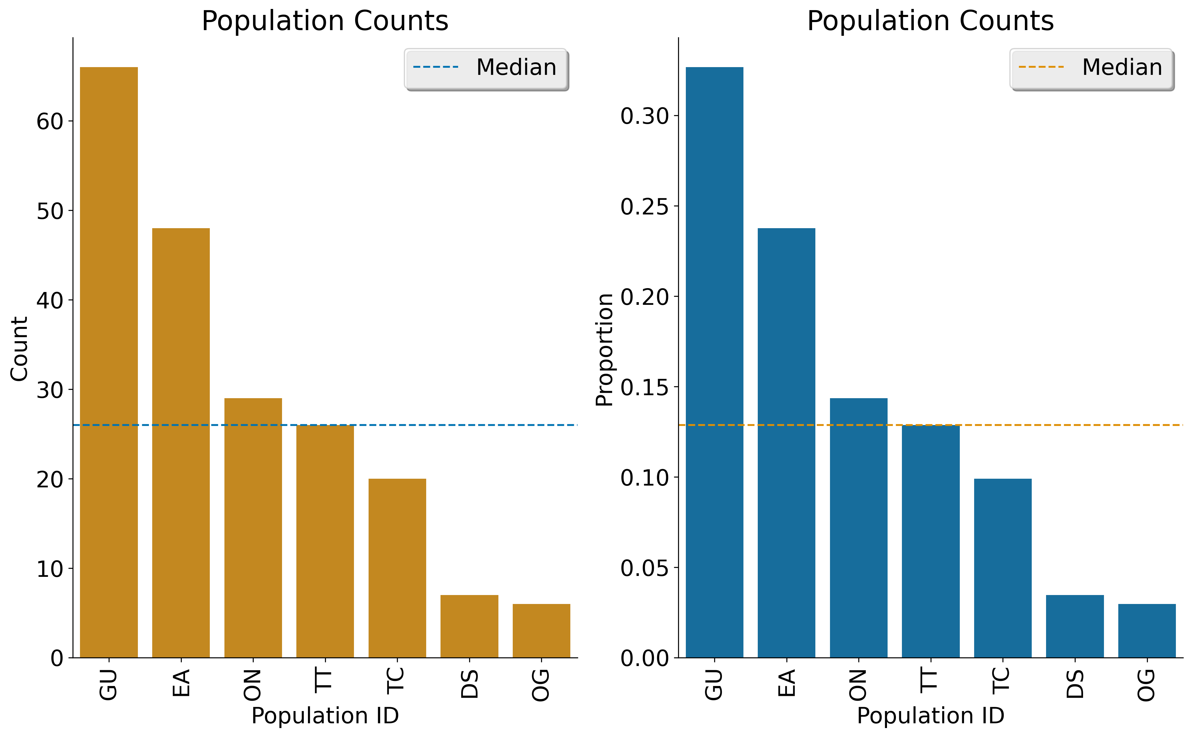
- The
GenotypeDataclass will automatically create a plot showing the number of inidviduals present in each population, if apopmapfileis provided. For example:
NRemover2 provides a variety of filtering methods to clean your genotype data. Here is an example of how to apply filters to remove samples and loci with too much missing data, monomorphic sites, singletons, minor allele count (MAC), minor allele frequency (MAF), and more:
# Apply filters to remove samples and loci with too much missing data
gd_filt = nrm.filter_missing_sample(0.75)
             .filter_missing(0.75)
             .filter_missing_pop(0.75)
             .filter_mac(2)
             .filter_monomorphic(exclude_heterozygous=False)
             .filter_singletons(exclude_heterozygous=False)
             .filter_biallelic(exclude_heterozygous=False)
             .resolve()

# Write the filtered VCF to a new file
gd_filt.write_vcf("filtered_output.vcf")filter_missing_sample(threshold): Filters samples with missing data
above the threshold.
filter_missing(threshold): Filters loci with missing data above the
threshold.
filter_missing_pop(threshold): Filters loci where missing data for any
given population is above the threshold.
filter_mac(threshold): Filters loci with a minor allele count below
the threshold.
filter_maf(threshold): Filters loci with a minor allele frequency
below the threshold.
filter_monomorphic(exclude_heterozygous): Filters monomorphic loci
(sites with only one allele).
filter_singletons(exclude_heterozygous): Filters singletons (sites
with only one occurrence of an allele).
filter_biallelic(exclude_heterozygous): Filters biallelic loci (sites
with only two alleles).
thin_loci(size): Thins loci by removing loci within size bases of
each other on the same locus or chromosome (based on input VCF CHROM
and POS fields). Note that this method only works with VCFReader and
is not available for PhylipReader and StructureReader. For example,
thin_loci(100) will remove all but one locus within 100 bases of eaach
other on the same chromosome.
filter_linked(size): Filters loci that are linked to other loci within
a specified distance (size), only considering the CHROM field from the
VCF file and ignoring the POS field. This method only works with
VCFReader and is not available for PhylipReader and StructureReader.
random_subset_loci(size): Randomly selects size number of loci from
the input dataset, where size is an integer.
resolve(): Applies the filters and returns the filtered GenotypeData
object. This method must be called at the end of the filtering chain to
apply the filters.
Note:
You must call resolve() at the end of the filtering chain to apply the
filters and return the filtered GenotypeData object.
Note:
The exclude_heterozygous parameter in filter_monomorphic,
filter_singletons, and filter_biallelic methods allows you to
exclude heterozygous genotypes from the filtering process. By default,
heterozygous genotypes are included in the filtering process.
Note:
thin_loci and filter_linked are only available for VCFReader and not
for PhylipReader and StructureReader.
Warning:
The filter_linked(size) method might yield a limited number of loci
with SNP data. It is recommended to use this method with caution and
check the output carefully.
search_thresholds() searches a range of filtering thresholds for all
missing data, minor allele frequency (MAF), and minor allele count (MAC)
filters. This method helps you find the optimal thresholds for your
dataset. It will plot the threshold search results so you can visualize
the impact of different thresholds on the dataset.
With search_thresholds(), you can specify the thresholds to search for
and the order in which to apply the filters:
# Initialize NRemover2 with GenotypeData object
nrm = NRemover2(gd)

# Specify filtering thresholds and order of filters
nrm.search_thresholds(
    thresholds=[0.25, 0.5, 0.75, 1.0],
    maf_thresholds=[0.01, 0.05],
    mac_thresholds=[2, 5],
    filter_order=[
        "filter_missing_sample",
        "filter_missing",
        "filter_missing_pop",
        "filter_mac",
        "filter_monomorphic",
        "filter_singletons",
        "filter_biallelic"
    ]
)
The search_thresholds() method will search for the optimal thresholds
for missing data, MAF, and MAC filters based on the specified thresholds
and filter order. It will plot the results so you can visualize the
impact of different thresholds on the dataset.
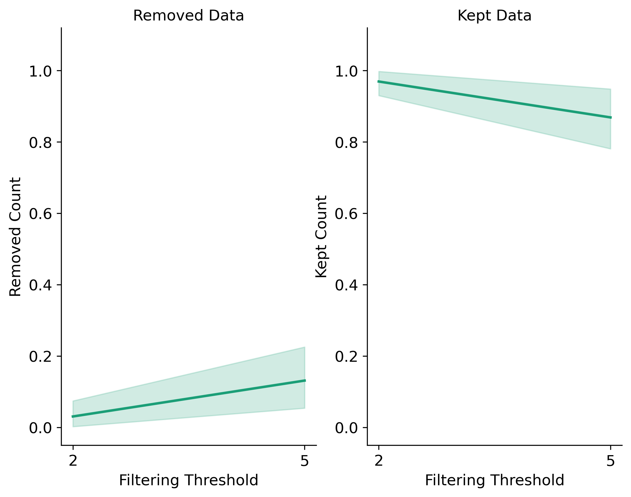
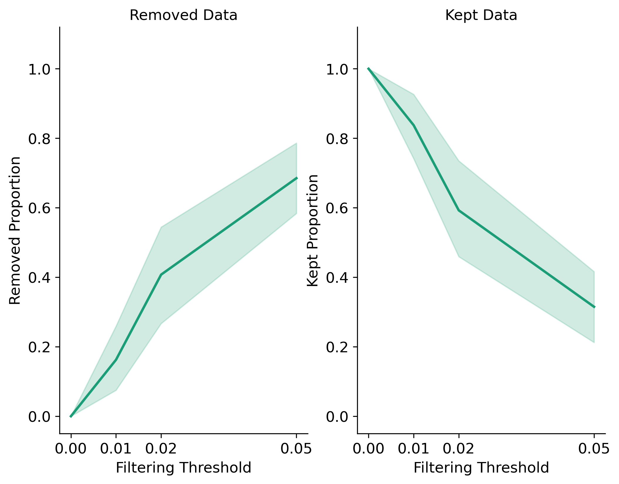
Below are example plots that are created when running the
search_thresholds() method:
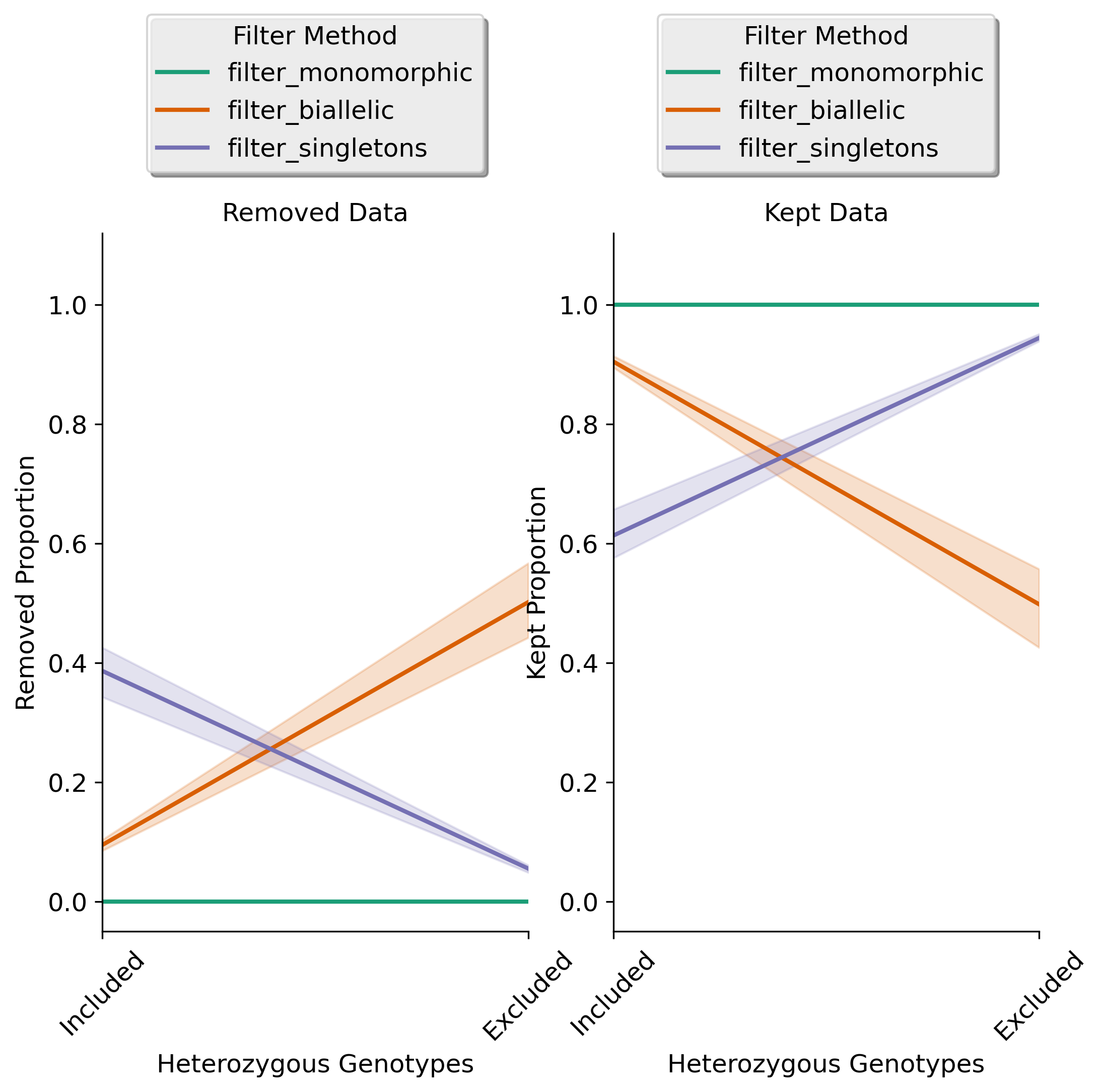
Filtering Results for Singletons, Monomorphic Sites, and Biallelic Sites:
Filtering Results for Minor Allele Count (MAC):
Filtering Results for Minor Allele Frequency:
Missing Data Filtering for Loci and Samples:
Missing Data Filtering for Populations:
Note:
The search_thresholds() method is incompatible with thin_loci(size)
and filter_linked() being in the filter_order list.
Warning:
The search_thresholds() method can also be called either before or
after any other filtering, but note that it will reset the filtering
chain to the original state.
plot_sankey_filtering_report() generates a Sankey plot to visualize
how SNPs are filtered at each step of the pipeline. For example:
from snpio import NRemover2, VCFReader

vcf = "snpio/example_data/vcf_files/phylogen_subset14K_sorted.vcf.gz"
popmap = "snpio/example_data/popmaps/phylogen_nomx.popmap"

gd = VCFReader(
    filename=vcf,
    popmapfile=popmap,
    force_popmap=True,
    verbose=True,
    plot_format="png",
    plot_fontsize=20,
    plot_dpi=300,
    despine=True,
    prefix="snpio_example"
)

# Initialize NRemover2.
nrm = NRemover2(gd)

# Apply filters to remove samples and loci.
gd_filt = nrm.filter_missing_sample(0.75)
             .filter_missing(0.75)
             .filter_missing_pop(0.75)
             .filter_mac(2)
             .filter_monomorphic(exclude_heterozygous=False)
             .filter_singletons(exclude_heterozygous=False)
             .filter_biallelic(exclude_heterozygous=False)
             .resolve()

nrm.plot_sankey_filtering_report()
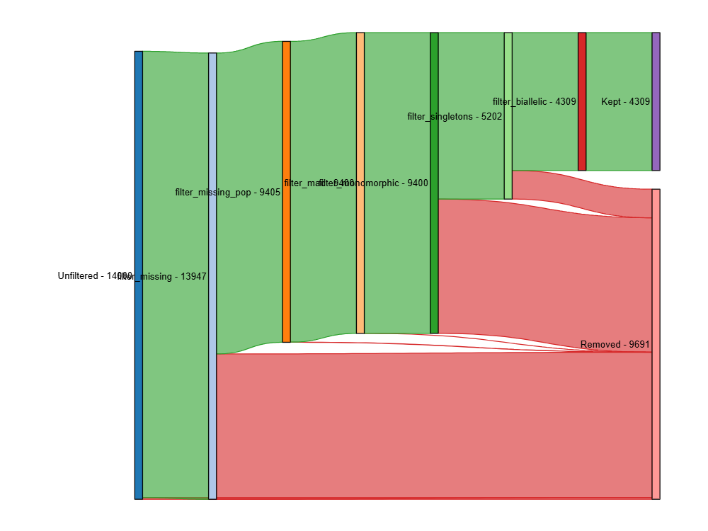
This will automatically track the number of loci at each filtering step and generate a Sankey plot to visualize the filtering process. The Sankey plot shows how many loci are removed at each step of the filtering process. For example:
In the Sankey Diagram above, the green nodes represent the number of loci remaining after each filtering step, and the red nodes represent the number of loci removed at each filtering step. The size of each edge is proportional to the number of loci retained or removed at each step. The Sankey plot provides a visual representation of the filtering process and helps you understand how each filtering method affects the dataset. The filtering order is dynamic based on the order each method was called.
Note:
The plot_sankey_filtering_report() must be called after filtering and
calling the resolve() method to generate the Sankey plot. It is also
incompatible with thin_loci(), filter_linked(), and
random_subset_loci() being in the filter_order list.
plot_sankey_filtering_report() only plots loci removed at each
filtering step and does not plot samples removed.
Once genotype data is loaded using any of the readers, you can access
several useful properties from the GenotypeData object:
num_snps: Number of SNPs or loci in the dataset.
num_inds: Number of individuals in the dataset.
populations: List of populations in the dataset.
popmap: Mapping of SampleIDs to PopulationIDs.
popmap_inverse: Dictionary with population IDs as keys and lists of
samples as values.
samples: List of samples in the dataset.
snpsdict: Dictionary with sampleIDs as keys and genotypes as values.
loci_indices: Numpy array with boolean values indicating the loci that
passed the filtering criteria set to True.
sample_indices: Numpy arrray with boolean values indicating the
samples that passed the filtering criteria set to True.
snp_data: 2D numpy array of SNP data of shape (num_inds, num_snps).
ref: List of reference alleles for each locus.
alt: List of alternate alleles for each locus.
inputs: Dictionary of input parameters used to load the genotype data.
SNPio also includes the GenotypeEncoder class for encoding genotype data into formats useful for downstream analysis and commonly used for machine and deep learning tasks.
The GenotypeEncoder class provides three encoding properties:
genotypes_onehot: Encodes genotype data into one-hot encoding, where
each possible biallelic IUPAC genotype is represented by a one-hot
vector. Heterozygotes are represented as multi-label vectors as follows:
onehot_dict = {
  "A": [1.0, 0.0, 0.0, 0.0],
  "T": [0.0, 1.0, 0.0, 0.0],
  "G": [0.0, 0.0, 1.0, 0.0],
  "C": [0.0, 0.0, 0.0, 1.0],
  "N": [0.0, 0.0, 0.0, 0.0],
  "W": [0.5, 0.5, 0.0, 0.0],
  "R": [0.5, 0.0, 0.5, 0.0],
  "M": [0.5, 0.0, 0.0, 0.5],
  "K": [0.0, 0.5, 0.5, 0.0],
  "Y": [0.0, 0.5, 0.0, 0.5],
  "S": [0.0, 0.0, 0.5, 0.5],
  "N": [0.0, 0.0, 0.0, 0.0],
}genotypes_int: Encodes genotype data into integer encoding, where each
possible biallelic IUPAC genotype is represented by an integer as
follows: as follows:
A=0, T=1, G=2, C=3, W=4, R=5, M=6, K=7, Y=8, S=9, N=-9.
genotypes_012: Encodes genotype data into 0-1-2 encoding, where 0
represents the homozygous reference genotype, 1 represents the
heterozygous genotype, and 2 represents the homozygous alternate
genotype.
Example Usage:
from snpio import VCFReader, GenotypeEncoder

vcf = "snpio/example_data/vcf_files/phylogen_subset14K_sorted.vcf.gz"
popmap = "snpio/example_data/popmaps/phylogen_nomx.popmap"

gd = VCFReader(
    filename=vcf,
    popmapfile=popmap,
    force_popmap=True,
    verbose=True,
    plot_format="png",
    plot_fontsize=20,
    plot_dpi=300,
    despine=True,
    prefix="snpio_example"
)

encoder = GenotypeEncoder(gd)

# Convert genotype data to one-hot encoding
gt_ohe = encoder.genotypes_onehot

# Convert genotype data to integer encoding
gt_int = encoder.genotypes_int

# Convert genotype data to 0-1-2 encoding.
gt_012 = encoder.genotypes_012
The GenotypeEncoder allows you to seamlessly convert genotype data into different formats depending on your needs for analysis or machine learning workflows.
You can also inversely convert the encoded data back to the original genotypes by just setting the GenotypeEncoder properties to a new value. For example:
# Convert one-hot encoded data back to genotypes
encoder.genotypes_onehot = gt_ohe

# Convert integer encoded data back to genotypes
encoder.genotypes_int = gt_int

# Convert 0-1-2 encoded data back to genotypes
encoder.genotypes_012 = gt_012
This will automatically update the original genotype data in the
GenotypeData object and convert it to the original format stored in the
snp_data property of the GenotypeData object.
SNPio also provides a TreeParser class to load and parse phylogenetic trees in Newick and NEXUS formats. The TreeParser class can read and parse tree files, modify tree structures, draw trees, and save trees in different formats.
Here are some examples of how to load and parse a phylogenetic tree using the TreeParser class:
from snpio import TreeParser, VCFReader

vcf = "snpio/example_data/vcf_files/phylogen_subset14K_sorted.vcf.gz"
popmap = "snpio/example_data/popmaps/phylogen_nomx.popmap"

gd = VCFReader(
    filename=vcf,
    popmapfile=popmap,
    force_popmap=True,
    verbose=True,
    plot_format="pdf",
    plot_fontsize=20,
    plot_dpi=300,
    despine=True,
    prefix="snpio_example"
)

# Load a phylogenetic tree from a Newick file
tp = TreeParser(
    genotype_data=gd,
    treefile="snpio/example_data/trees/test.tre",
    siterates="snpio/example_data/trees/test14K.rates",
    qmatrix="snpio/example_data/trees/test.iqtree",
    verbose=True
)

tree = tp.read_tree()
tree.draw()  # Draw the tree

# Save the tree in Newick format
tp.write_tree(tree, save_path="snpio/example_data/trees/test_newick.tre")

# Save the tree in NEXUS format
tp.write_tree(tree, save_path="snpio/example_data/trees/test_nexus.nex", nexus=True)

# Returns the tree in Newick format as a string
tp.write_tree(tree, save_path=None)

# Get the tree stats. Returns a dictionary of tree stats.
print(tp.tree_stats())

# Reroot the tree at any nodes containing the string 'EA' in the sampleID.
# Use the '~' character to specify a regular expression pattern to match.
tp.reroot_tree("~EA")

# Get a distance matrix between all nodes in the tree.
print(tp.get_distance_matrix())

# Get the Rate Matrix Q from the Qmatrix file.
print(tp.qmat)

# Get the Site Rates from the Site Rates file.
print(tp.site_rates)

# Get a subtree with only the samples containing 'EA' in the sampleID.
# Use the '~' character to specify a regular expression pattern to select all
# tips containing the pattern.
subtree = tp.get_subtree("~EA")

# Prune the tree to remove samples containing 'ON' in the sampleID.
pruned_tree = tp.prune_tree("~ON")

# Write the subtree and pruned tree. Returns a Newick string if 'save_path'
# is None. Otherwise saves it to 'save_path'.
print(tp.write_tree(subtree, save_path=None))
print(tp.write_tree(pruned_tree, save_path=None))
The TreeParser class provides several methods for working with phylogenetic trees, including reading, writing, and modifying trees. You can use these methods to analyze and manipulate phylogenetic trees for your research and analysis tasks.
The TreeParser class also provides methods for calculating tree statistics, rerooting trees, getting distance matrices, and extracting subtrees based on sample IDs. These methods can help you analyze and visualize phylogenetic trees and extract relevant information for downstream analysis.
The Rate matrix Q and Site Rates can be accessed from the Qmatrix and Site Rates files, respectively. These matrices can be used to calculate evolutionary distances and rates between samples in the phylogenetic tree. The siterates file can be output by IQ-TREE or specified as a one-column file with the rates for each site in the alignment (header optional). The qmatrix file can be obtained from the IQ-TREE standard output (.iqtree file) or from a stand-alone Qmatrix file with the rate matrix Q. In the latter case, the file should be a tab-delimited or comma-delimited file with the rate matrix Q with substitution rates in the order: "A, "C", "G", "T". A header line is optional.
The rate matrix and site rates objects can be accessed by their corresponding properties:
tp.qmat: Rate matrix Q.tp.site_rates: Site rates.
For more information on the TreeParser class and its methods, please refer to the API documentation.
You can benchmark the filtering performance using the Benchmark class to visualize how thresholds affect the dataset, if you have installed the snpio dev requirements:
pip install snpio[dev]Then, you can use the Benchmark class to plot performance metrics for
your filtered genotype data after the resolve() method is called. For
example:
from snpio.utils.benchmarking import Benchmark

Benchmark.plot_performance(nrm.genotype_data, nrm.genotype_data.resource_data)
This function will plot performance metrics for your filtered genotype
data and for the VCFReader class, giving insights into data quality
changes.
For more information on the Benchmark class and how to use it, see the API documentation.
This guide provides an overview of how to get started with the SNPio library. It covers the basic steps to read, manipulate, and analyze genotype data using the VCFReader, PhylipReader, StructureReader, and NRemover2 classes. SNPio is designed to simplify the process of handling genotype data and preparing it for downstream analysis, such as population genetics, phylogenetics, and machine learning. The library supports various file formats, including VCF, PHYLIP, and STRUCTURE, and provides tools for filtering, encoding, and visualizing genotype data. This guide will help you get up and running with SNPio quickly and efficiently.
For more information on the SNPio library, please refer to the API documentation and examples provided in the repository. If you have any questions or feedback, please feel free to reach out to the developers.
We hope you find SNPio useful for your bioinformatic analyses!
Note:
The SNPio library is under active development, and we welcome contributions from the community. If you would like to contribute to the project, please check the GitHub repository for open issues and submit a pull request. We appreciate your support and feedback!
If you encounter any issues or have any questions about the SNPio library, please feel free to reach out to the developers or open an issue on the GitHub repository. We are here to help and improve the library based on your feedback.
The SNPio library is licensed under the GPL3 License, and we encourage you to use it for your research and analysis tasks. If you find the library useful, please cite it in your publications. We appreciate your support and feedback!
