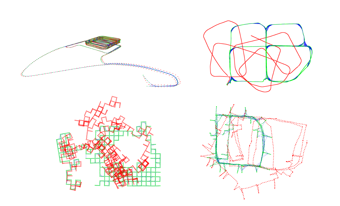
 Figure 1: Example Results Visualization. More examples can be found here.
- Features
- For an education purpose
- From-scratch pose-graph optimization implementation
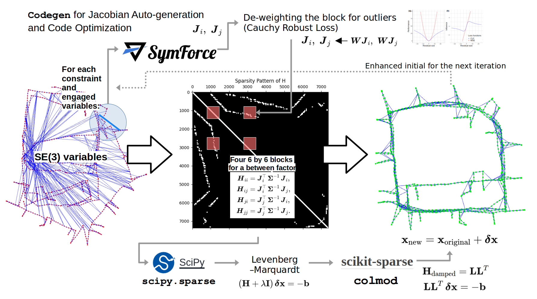
- This tried to maximize the code-level transparency of the process of generating the H and b matrices, building a linear system, and controlling the LM iterations.
- A single file
- Miminum dependencies: numpy/scipy/symforce/sksparse (and open3d for visualization).
- numpy for basic matrix handling
- scipy for basic rotation functions and sparse matrix containers
- symforce for the auto-generated symbolic Jacobian (optional)
- sksparse for cholmod and solve function
- open3d for large-sized point cloud (pose-graph) visualization
- I hope this hands-on tutorial code can also be used as training material for Symforce's auto-generated optimized Jacobian code generation (codegen).
- For the details, see below Symforce-based Auto-generated Jacobians.
- ps. This tutorial supports only batch pose-graph optimization (but with a sparse solver!) and does not cover incrementally expanding pose-graph optimization (e.g., iSAM).
 Figure 2: The pipeline of nano-pgo
- Recommend to use python<3.12 and numpy<2, for example,
$ python3.11 -m venv ~/envs/py311$ source ~/envs/py311/bin/activate$ pip install "numpy<2.0"$ pip install scipy$ sudo apt-get install libsuitesparse-dev$ pip install scikit-sparse$ pip install symforce$ pip install matplotlib$ pip install open3d
$ python nano_pgo.py- It's also recommended to compare the results from GTSAM (better and faster!) by using
baseline_gtsam.py.
- It's also recommended to compare the results from GTSAM (better and faster!) by using
- Note that the nano_pgo.py's goal is a maximized transparency of all logics and theories from state representations to building and solving linear systems.
- Demo video can be found here.
- Understand
- what is pose-graph optimization.
- what is a g2o-format pose-graph data.
- what is se(3) and SE(3) (the tangent space and the manifold).
- what is iterative least-square optimization and solving normal equation.
- what is the error and jacobians of between factors and how to be derived.
- what is the gauge freedom of pose-graph SLAM.
- why sparse solver is necessary (here, we used sksparse.cholmod).
- why damping is necessary (i.e., LM iterative optimization method).
- why robust loss is necessary (here, we used Cauchy deweighting).
- what are the differences between numerical and symbolic diffs.
- how to use symforce APIs.
- how to use GTSAM APIs.
- what is the real-world problems, use-cases, and state-of-the arts.
-
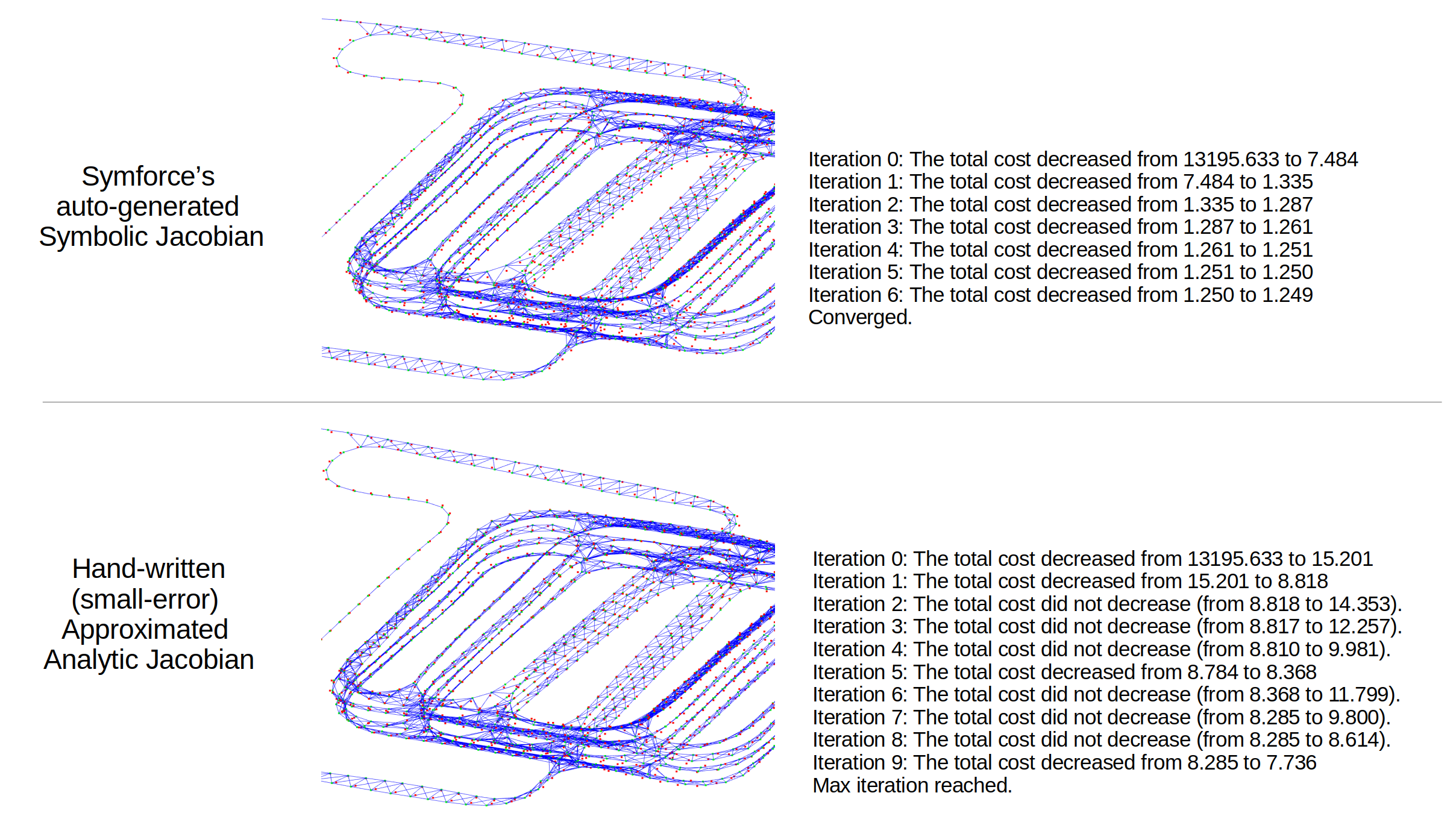
SymForce eliminates the need for tedious and error-prone manual Jacobian derivations.
-
You can enjoy this feature by setting
self.use_symforce_generated_jacobian=Trueanddebug_compare_jacobians=True. Figure 3: Auto-generated Symbolic Jacobian's effectiveness.
 -
You can first automatically generate the (symbolic) Jacobian of the relative SE(3) error like this,
import symforce.symbolic as sf
from symforce.ops import LieGroupOps

# Define rotation variables (rotation vectors for each axis)
sf_ri = sf.V3.symbolic("ri")  # Rotation of pose_i
sf_rj = sf.V3.symbolic("rj")  # Rotation of pose_j
sf_rij = sf.V3.symbolic("rij")  # Measured relative rotation

# Define translation variables
sf_ti = sf.V3.symbolic("ti")  # Translation of pose_i
sf_tj = sf.V3.symbolic("tj")  # Translation of pose_j
sf_tij = sf.V3.symbolic("tij")  # Measured relative translation

# Create rotation matrices using Lie Group operations
sf_Ri = LieGroupOps.from_tangent(sf.Rot3, sf_ri)
sf_Rj = LieGroupOps.from_tangent(sf.Rot3, sf_rj)
sf_Rij = LieGroupOps.from_tangent(sf.Rot3, sf_rij)

# Construct SE(3) containers
sf_Ti = sf.Pose3(R=sf_Ri, t=sf_ti)
sf_Tj = sf.Pose3(R=sf_Rj, t=sf_tj)
sf_Tij = sf.Pose3(R=sf_Rij, t=sf_tij)

# SE3 error: T_err = T_ij^{-1} * T_i^{-1} * T_j
sf_T_err = sf_Tij.inverse() * (sf_Ti.inverse() * sf_Tj)

# Convert SE3 error to a tangent vector [r, t], 6-dim.
#  NOTE: symforce uses the [r, t] order, not [t, r].
sf_se3_err = sf.Matrix(sf_T_err.to_tangent())

# Define residual as the rotation and translation error
sf_residual = sf_se3_err  # 6D vector

# Compute the full Jacobian
sf_J_ti = sf_residual.jacobian([sf_ti])  # 6 x 3
sf_J_ri = sf_residual.jacobian([sf_ri])  # 6 x 3
sf_J_tj = sf_residual.jacobian([sf_tj])  # 6 x 3
sf_J_rj = sf_residual.jacobian([sf_rj])  # 6 x 3
-
Then, next step is to inject (evaluate) the actual values to the symbolic (block of) Jacobian functions, like
def between_factor_jacobian_by_symforce(pose_i, pose_j, pose_ij_meas):
    """
    Computes the Jacobians for the between factor residual using Symforce symbolic computation.

    Parameters:
        pose_i (dict): Dictionary containing rotation vector 'r' and translation 't' for pose i.
        pose_j (dict): Dictionary containing rotation vector 'r' and translation 't' for pose j.
        pose_ij_meas (dict): Dictionary containing the measured relative rotation matrix 'R' and translation vector 't'.

    Returns:
        Ji (np.ndarray): 6x6 Jacobian matrix with respect to pose i.
        Jj (np.ndarray): 6x6 Jacobian matrix with respect to pose j.

    Note: the Ji and Jj should have shapes (6, 6) like:
                                        |  translation_variable (3-dim), rotation_variable (3-dim) |
            cost_func_translation_part  |               *                          *               |
            cost_func_rotation_part     |               *                          *               |
    """

    substitutions = {
        sf_ri: sf.V3(pose_i["r"] + epsilon),
        sf_ti: sf.V3(pose_i["t"] + epsilon),
        sf_rj: sf.V3(pose_j["r"] + epsilon),
        sf_tj: sf.V3(pose_j["t"] + epsilon),
        sf_rij: sf.V3(rotmat_to_rotvec(pose_ij_meas["R"]) + epsilon),
        sf_tij: sf.V3(pose_ij_meas["t"] + epsilon),
    }

    sf_J_ti_val = sf_J_ti.subs(substitutions).to_numpy()
    sf_J_ri_val = sf_J_ri.subs(substitutions).to_numpy()
    sf_J_tj_val = sf_J_tj.subs(substitutions).to_numpy()
    sf_J_rj_val = sf_J_rj.subs(substitutions).to_numpy()

    # ps. the reason why the index 3: mapped to :3
    # is because this example uses [t, r], but symforce uses the order of [r, t]
    sf_Ji = np.zeros((6, 6))
    sf_Ji[:3, :3] = sf_J_ti_val[3:, :]
    sf_Ji[3:, :3] = sf_J_ti_val[:3, :]
    sf_Ji[:3, 3:] = sf_J_ri_val[3:, :]
    sf_Ji[3:, 3:] = sf_J_ri_val[:3, :]

    sf_Jj = np.zeros((6, 6))
    sf_Jj[:3, :3] = sf_J_tj_val[3:, :]
    sf_Jj[3:, :3] = sf_J_tj_val[:3, :]
    sf_Jj[:3, 3:] = sf_J_rj_val[3:, :]
    sf_Jj[3:, 3:] = sf_J_rj_val[:3, :]

    return sf_Ji, sf_Jj
-
However, the above "raw" symbolic Jacobian includes many redundant computations, making it slow. Therefore, by using SymForce's codegen functionality, it is possible to perform compilation and code optimization (i.e., compile the Jacobian), resulting in more than a 30x speed improvement in raw Python (here, for a single block calculation, that is a single edge's H and b, 0.0031 sec to 0.00009 sec, at a single core of AMD Ryzen 7 8845HS CPU). An example of using the Symforce
codegenAPI is like:# optimized code compliation process def sf_between_error(Ti: sf.Pose3, Tj: sf.Pose3, Tij: sf.Pose3): return Tij.inverse() * (Ti.inverse() * Tj) between_error_codegen = codegen.Codegen.function( func=sf_between_error, config=codegen.PythonConfig(), ) between_error_codegen_with_jacobians = between_error_codegen.with_jacobians( which_args=["Ti", "Tj"], include_results=True, ) between_error_codegen_with_jacobians_data = ( between_error_codegen_with_jacobians.generate_function() ) # copy the generated source file and import ... # ... # Then you can use like this # (Using the above auto-geneated functions within the copied __between_error_codegen.py file) _, res_D_Ti, res_D_Tj = sf_between_error_with_jacobians01( Ti=sym.Pose3(R=sym.rot3.Rot3(rotvec_to_quat(pose_i["r"])), t=pose_i["t"]), Tj=sym.Pose3(R=sym.rot3.Rot3(rotvec_to_quat(pose_j["r"])), t=pose_j["t"]), Tij=sym.Pose3( R=sym.rot3.Rot3(rotvec_to_quat(pose_ij_meas["r"])), t=pose_ij_meas["t"], ), ) # see `between_factor_jacobian_by_symforce` function in the `nano_pgo.py` for the details.
- Equipped with better initialization strategies (e.g., rotation averaging)
- Detailed teaching materials
- Datasets from https://lucacarlone.mit.edu/datasets/