A Python 3 script for easy calibration of ⁵⁷Fe-Mößbauer (MB) spectra from a ⁵⁷Fe sample.
lmfit
numpy
scipy
matplotlib
Start the script with:
python3 cal-mb.py 57Fe_calib_raw_data.ws5calculates the folding point FP, v0 (channel where the velocity is zero),
vmax (maximum velocity), and the velocity / channel f.
The file should contain intensities or counts from a multi-channel analyzer. The popular WissEl
format has the extension .ws5. In principle any raw data (not only WissEl) can be processed. Pay
attention to the start channel number and the folding direction.
Terminal output:
======================================
Results for 57Fe_calib_raw_data.ws5 :     ⇦ name of the file that contains the ⁵⁷Fe-MB-spectrum
File modified on 24.08.2023 13:33:53      ⇦ modification date
--------------------------------------
FP (channel) = 256.7889±0.0588            ⇦ folding point
v₀ (channel) = 125.6873±0.0620            ⇦ channel where velocity is zero
vmax /mm·s⁻¹ =  -4.6926±0.0111            ⇦ maximum velocity
f /mm·s⁻¹/c  =   0.0368±0.0001            ⇦ velocity / channel
======================================
Statistics (folded data with weights):
--------------------------------------
data points :  256                        ⇦ number of data points
variables   :  13                         ⇦ number of variables
mean σ data :  152.68                     ⇦ weights for χ² and red. χ²
χ²          :  537.49                     ⇦ Chi square(d)
red. χ²     :  2.21                       ⇦ reduced Chi square(d)
R²          :  0.9736                     ⇦ R square(d)
======================================
You can use the first three parameters to fit MB spectra with fit-mb.
Start the script with:
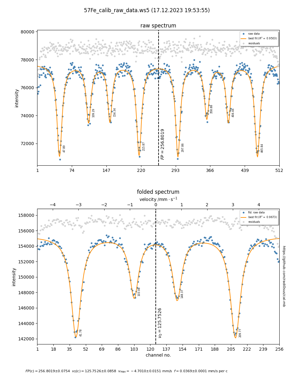
python3 cal-mb.py 57Fe_calib_raw_data.ws5 -scalculates the same values as described above. In addition a matplotlib window is shown that
summarizes the fit results.
The results will not be saved. To keep the output you have to start the script with:
python3 cal-mb.py 57Fe_calib_raw_data.ws5 > calib_from_today.txtTo keep the figure, you have to click the floppy symbol (similar to 💾) in the matplotlib window.
- The script is benchmarked against the
mcalprogram from Dr. Eckhard Bill. Within the given restrictions, the results match quite well. - Raw spectra (WissEl .ws5 for example) are expected to start at channel 1 and be folded to the right.
- With the
-floption the raw spectrum can be folded to the left. -
FPis the mean of the centers of the individual Lorentz functions (4, 8 or 12) of the raw spectrum. -
v0is the mean of the centers of the individual Lorentz functions (2, 4 or 6) of the folded spectrum. -
fis the mean offcalculated with$\Delta E_Q$ from ⁵⁷Fe divided by the difference of the centers of the single Lorentz functions from the outermost to the innermost pair (see also comment in the script). -
vmaxisf * 127.5in case of 256 channels. - In case of unfolded data, the error can be estimated from the differences in the intensities of the left-hand side and
right-hand side sub-spectra. The weighting for χ² and red. χ² is 1 / (mean standard deviation).
The mean standard deviation is the square root of the mean variance of two times the intensities of the left-hand side
and right-hand side data pairs which are supposed to be equal. χ² should be close to the number of data points and red. χ²
should close to 1 in case of a good fit.
Please note that the calibration parameters are mainly derived from channel or velocity data (x-values), while only errors from intensity data or counts (y-values) are taken into account for the weigths of χ² and red. χ². - R² is calculated by 1 - variance(residual * mean standard deviation) / variance(intensities or counts),
because R² is calculated wrongly by
lmfitin case of weights. - All other values and errors are calculated with
lmfit. - The script has not been tested with raw data from 1024 channel multi-channel analyzers.

