Based on Nvidia End-to-End Learning model here
The project uses the simulator developed by Udacity as present in this repository. The dataset for training has also been generated using the same.
- Nvidia CUDA Toolkit 11.0 download
- Tensorflow 2.5 Nightly environment with support for Nvidia CUDA 11
conda create -n tf-n-gpu python conda activate tf-n-gpu pip install tf-nightly-gpu - MoviePy
conda install -c conda-forge moviepy - Eventlet
conda install -c conda-forge eventlet - SocketIO
conda install -c conda-forge python-socketio - CuDNN
conda install -c anaconda cudnn - NumPy
conda install -c anaconda numpy - Matplotlib
conda install -c conda-forge matplotlib
Consider using the requirements.txt for easy installation of Dependencies.
From inside an activated tensorflow environment, run the following commands on Anaconda Prompt:
- Train:
python model.py
This creates the model.h5 file (also present in the repository) - Test on simulator:
python drive.py model.h5 images
This runs the trained model. After the socket starts listening, start the simulator software, and select Autonomous Mode The car should start driving autonomously based on the trained model. The frames from this run will be recorded, and stored in a folder titled images in the project directory. - Stitch the output frames into a cohesive video:
python video.py images --fps 75
The video by default is created at 60 fps, if fps is not passed.
| Layer | Description |
|---|---|
| Input | 160 x 320 x 3 RGB image |
| Cropping | Eliminates irrelevant data such as sky and environment |
| Lambda | Resizes the input to fit the model's requirement |
| Normalization | |
| Convolution 5x5 | 2x2 stride, activation = 'relu', filters = 24 |
| Convolution 5x5 | 2x2 stride, activation = 'relu', filters = 36 |
| Convolution 5x5 | 2x2 stride, activation = 'relu', filters = 48 |
| Convolution 3x3 | 1x1 stride, activation = 'relu', filters = 64 |
| Convolution 3x3 | 1x1 stride, activation = 'relu', filters = 64 |
| Flatten | |
| Fully Connected | 100, activation = 'relu' |
| Fully Connected | 50, activation = 'relu' |
| Fully Connected | 10, activation = 'relu' |
| Fully Connected | 1, activation = 'linear' |
My model consists of a convolution neural network with a combination of 3x3 filters and 5x5 filters and depths between 24 and 64 (model.py lines 80-84). This is identical to the model proposed by NVIDIA. Some of the layers use striding while others don't.
The model includes RELU layers to introduce nonlinearity (model.py lines 80-84), and the data is normalized in the model using a Keras LayerNormalization layer (model.py line 79). Cropping has also been incorporated into the network itself, to ensure a better model by eliminating areas of non-importance. My research suggests the validation loss increased when cropping is also used towards the bottom of the image, and so it has been skipped.
The model generalizes well by default, as a result of strided convolutions and well augmented data, and does not need additional measures to reduce overfitting. Augmentation steps included flipping the training data, as well as incorporating images from all three cameras.
The model was tested by running it through the simulator and ensuring that the vehicle could stay on the track. Increasing the speed made poorer models wobbly, but eventually I was able to stabilize the model even at maximum speed available in the simulator.
Checkpointing using validation loss(model.py line 93) and Early Stopping with a patience of 10 (model.py line 94) has been implemented to ensure we save the best model that has been trained.
The model used an Adam optimizer, optimized using Exponential Decayed learning rate (model.py lines 96-97) to ensure better convergence.
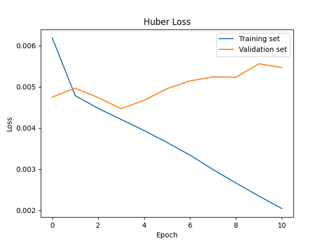
Huber Loss has been incorporated (model.py line 98) because it performed better than other experimented loss functions for Regression Models such as MSE.
20% of the training data has been used for validation, and shuffling of data has been incorporated inside the fit() call (model.py line 102).
Training data was chosen to keep the vehicle driving on the road. I used a combination of center lane driving, recovering from the left and right sides of the road using a correction factor of 0.2.
For details about how I created the training data, see the next section.
The overall strategy for deriving a model architecture was to design a convolutional model that could work effectively for my use case.
My first step was to use a convolution neural network model similar to the NVIDIA End-To-End Model for Self Driving Cars. I thought this model might be appropriate because it has already been optimized for self driving cars and fit my use case accurately. I initially tried training using much larger models such as Inception_V3 (22M parameters) and NASNetLarge (85M parameters). However, they failed to produce satisfactory results when used in my application.
In order to gauge how well the model was working, I split my image and steering angle data into a training and validation set. I found that my first model had a low loss on the training set and a low loss on the validation set. This implied that the model was underfitting, and not training.
Throughout the process of debugging the program, I discovered much about regression models: that classification-specific metrics such as Accuracy don't work for Regression, and final activation functions need to be changed from softmax and ReLU to linear. I having little experience with regression models before found these observations profound, and getting these concepts cleared helped me optimize the model.
To combat the underfit model, I eliminated all the dropout layers I had initially designed for it. Then, I optimized the initial learning rate for the Exponential Decay, to make it suit my model much better.
The final step was to run the simulator to see how well the car was driving around track one. The initial underfit models produced a constant steering angle of -25 degrees, before I had changed the final activation function from ReLU to Linear. Afterwards, tuning more parameters such as initial learning rate helped my model get more robust.
At the end of the process, the vehicle is able to drive autonomously around the track without leaving the road at the maximum speed possible.
The final model architecture (model.py lines 76-89) consisted of a convolution neural network with the following layers and layer sizes.
Here is a visualization of the architecture
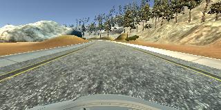
To capture good driving behavior, I first recorded two laps on track one using center lane driving. Here is an example image of center lane driving:
I then recorded the vehicle recovering from the left side and right sides of the road back to center so that the vehicle would learn to recover if it ever finds itself not positioned in the center. I made selective recordings of only when the vehicle moves towards the center and not when the vehicle moves away from the center. This ensured the vehicle never was trained to move away from the center. I also generated one batch of training data by driving the vehicle in reverse in the same circuit, thereby negating the bias towards left that was induced by the circuit, which had more left turns than right turns.
I did not repeat this process on track two, since it was inversely affecting my model. Since my model does not exactly account for varying heights, the difference in elevation confused the model during training and I found it increased the Huber Loss by approximately 0.003 points.
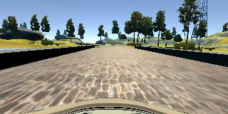
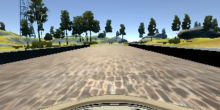
To augment the data sat, I also flipped images and angles thinking that this would make the model more robust. For example, here is an image that has then been flipped:
After the collection process, I had 48216 data points, out of which 38572 was used for training and 9644 used for validation. I had included preprocessing steps in my Netowrk Layers, such as Cropping and Normalization, so I did not implement any such measures externally.
I observed that shuffling the data externally decreased performance as compared to enabling shuffle inside model.fit() (model.py line 99), so I implemented it there itself. I have also implemented a validation split of 20% inside model.fit().
I used this training data for training the model. The validation set helped determine if the model was over or under fitting. The ideal number of epochs was 4 on average as evidenced by the Early Stopping Algorithm. I used an Adam optimizer so that manually training the learning rate wasn't necessary.
The Loss variations over epochs is visible through the following visualization:


