Alternating Minimization Based Trajectory Generation for Quadrotor Aggressive Flight
This repo is deprecated.
For local-planning, it is encouraged to use our EGO-Planner.
For general-purpose multicopter trajectory optimization, it is encouraged to check our solver GCOPTER if released.
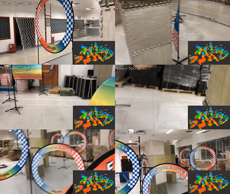
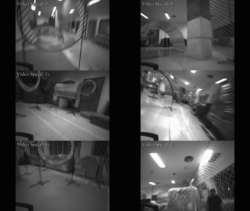
AM-Traj is a C++11 header-only library for generating large-scale piecewise polynomial trajectories for aggressive autonomous flights, with highlights on its superior computational efficiency and simultaneous spatial-temporal optimality. Besides, an extremely fast feasibility checker is designed for various kinds of constraints. All components in this framework leverage the algebraic convenience of polynomial trajectory optimization problem, thus our method is capable of computing a spatial-temporal optimal trajectory with 60 pieces within 5ms, i.e., 150Hz at least. You just need to include "am_traj.hpp" and "root_finder.hpp" in your code. Please use the up-to-date master branch which may have a better performance than the one in our paper.
Author: Zhepei Wang and Fei Gao from the ZJU Fast Lab.
Related Papers:
-
Alternating Minimization Based Trajectory Generation for Quadrotor Aggressive Flight, Zhepei Wang, Xin Zhou, Chao Xu, Jian Chu, and Fei Gao, IEEE Robotics and Automation Letters (RA-L).
-
Detailed Proofs of Alternating Minimization Based Trajectory Generation for Quadrotor Aggressive Flight, Zhepei Wang, Xin Zhou, Chao Xu, and Fei Gao, the supplementary material.
If you use our code for your academic research, please cite the first related paper.
Video Links: youtube or bilibili
-
Only two headers are required for usage. The first one is "am_traj.hpp", which contains a polynomial trajectory optimizer. The second one is "root_finder.hpp", which originates from a self-developed toolkit.
-
The library is able to generate large-scale trajectories with optimal coefficients and optimal time allocations in real-time, without using general purpose NLP solvers. Both the unconstrained case as well as the constrained case are considered.
-
The library provides an efficient formulation for various feasibility checkers. Only algebraic operations are involved, which make our feasbility check for some high-order (>4) constraints even faster than traditional check by closed-form solutions for low-order constraints (<=4). Therefore, the scalability makes it no longer painful to do feasibility check for high-order polynomial trajectories.
-
The library implements an extremely fast spatial trajectory solver when time allocation is prefixed and constraints are not considered. It uses a Banded LU Factorization which is much more efficient here than a general Sparse LU Factorization. The former has linear time complexity while the latter may get stuck in its "analyzePattern". Therefore, our lib only requires 4 (or 18) seconds to generate an Unconstrained Spatial (or Spatial-Temporal) Optimal Traj with 1000000 Segments!!!
Only three functions below are needed.
AmTraj(double wT, double wA, double wJ, double mVr, double mAr, int mIts, double eps)
Inputs:
wT: Weight for the time regularization
wA: Weight for the integrated squared norm of acceleration
wJ: Weight for the integrated squared norm of jerk
mVr: Maximum velocity rate
mAr: Maximum acceleration rate
mIts: Maximum number of iterations in optimization
eps: Relative tolerance
Outputs:
An instance of AmTraj: An object used for trajectory generation
Example:
AmTraj amTrajOpt(1024.0, 32.0, 1.0, 7.0, 3.5, 32, 0.02);
Trajectory AmTraj::genOptimalTrajDT(const std::vector<Eigen::Vector3d> &wayPs, Eigen::Vector3d iniVel, Eigen::Vector3d iniAcc, Eigen::Vector3d finVel, Eigen::Vector3d finAcc) const
Inputs:
wayPs: Fixed waypoints for a trajectory
iniVel: Trajectory velocity at the first waypoint
iniAcc: Trajectory acceleration at the first waypoint
finVel: Trajectory velocity at the last waypoint
finAcc: Trajectory acceleration at the last waypoint
Outputs:
An instance of Trajectory: A trajectory with optimal coefficient matrices and optimal durations, on which constraints of maximum velocity/acceleration rate are not guaranteed
Example:
Eigen::Vector3d iV(2.0, 1.0, 0.0), fV(0.0, 0.0, 0.0)
Eigen::Vector3d iA(0.0, 0.0, 2.0), fA(0.0, 0.0, 0.0)
std::vector<Eigen::Vector3d> wPs;
wPs.emplace_back(0.0, 0.0, 0.0);
wPs.emplace_back(4.0, 2.0, 1.0);
wPs.emplace_back(9.0, 7.0, 5.0);
wPs.emplace_back(1.0, 3.0, 2.0);
Trajectory traj = amTrajOpt.genOptimalTrajDT(wPs, iV, iA, fV, fA);
Trajectory AmTraj::genOptimalTrajDTC(const std::vector<Eigen::Vector3d> &wayPs, Eigen::Vector3d iniVel, Eigen::Vector3d iniAcc, Eigen::Vector3d finVel, Eigen::Vector3d finAcc) const
Inputs:
wayPs: Fixed waypoints for a trajectory
iniVel: Trajectory velocity at the first waypoint
iniAcc: Trajectory acceleration at the first waypoint
finVel: Trajectory velocity at the last waypoint
finAcc: Trajectory acceleration at the last waypoint
Outputs:
An instance of Trajectory: A trajectory with optimal coefficient matrices and best time allocation, whose maximum velocity/acceleration rate are guaranteed to satisfy constraints
Example:
Eigen::Vector3d iV(2.0, 1.0, 0.0), fV(0.0, 0.0, 0.0)
Eigen::Vector3d iA(0.0, 0.0, 2.0), fA(0.0, 0.0, 0.0)
std::vector<Eigen::Vector3d> wPs;
wPs.emplace_back(0.0, 0.0, 0.0);
wPs.emplace_back(4.0, 2.0, 1.0);
wPs.emplace_back(9.0, 7.0, 5.0);
wPs.emplace_back(1.0, 3.0, 2.0);
Trajectory traj = amTrajOpt.genOptimalTrajDTC(wPs, iV, iA, fV, fA);
There are many useful functions in the header files. Use it by following their comments.
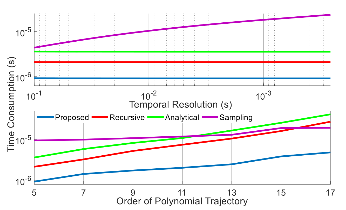
We compare our feasibility check method with Mueller's recursive bound check, Burri's analytical extrema check, as well as the widely used sampling-based check. In each case, 1000 trajectory pieces are randomly generated along with maximum velocity rate constraints to estimate average time consumption. As is shown in above figure, our method outperforms all other methods in computation speed because of its resolution independence and scalability with higher polynomial orders.
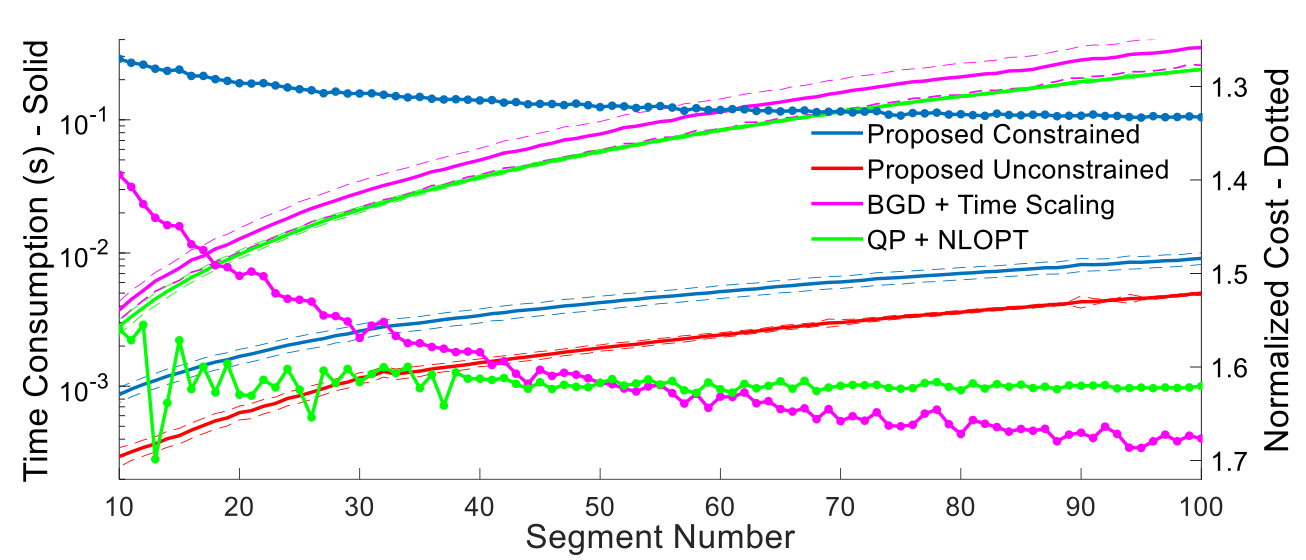
The benchmark is done as follows: We generate a sequence of waypoints by random walk, of which the step is uniformly distributed over [-3.0m, 8.0m] for each axis. The maximum speed and acceleration rates are set to 5.0m/s and 3.5m/s^2, respectively. The derivatives on the first and the last waypoints are set to zero. The objective function is set as wT=512.0, wA=0.0, wJ=1.0. For a given number of pieces, each method is applied to 1000 sequences of waypoints. The cost is then normalized by the cost of unconstrained case of our method. All comparisons are conducted on an Intel Core i7-8700 CPU under Linux environment.
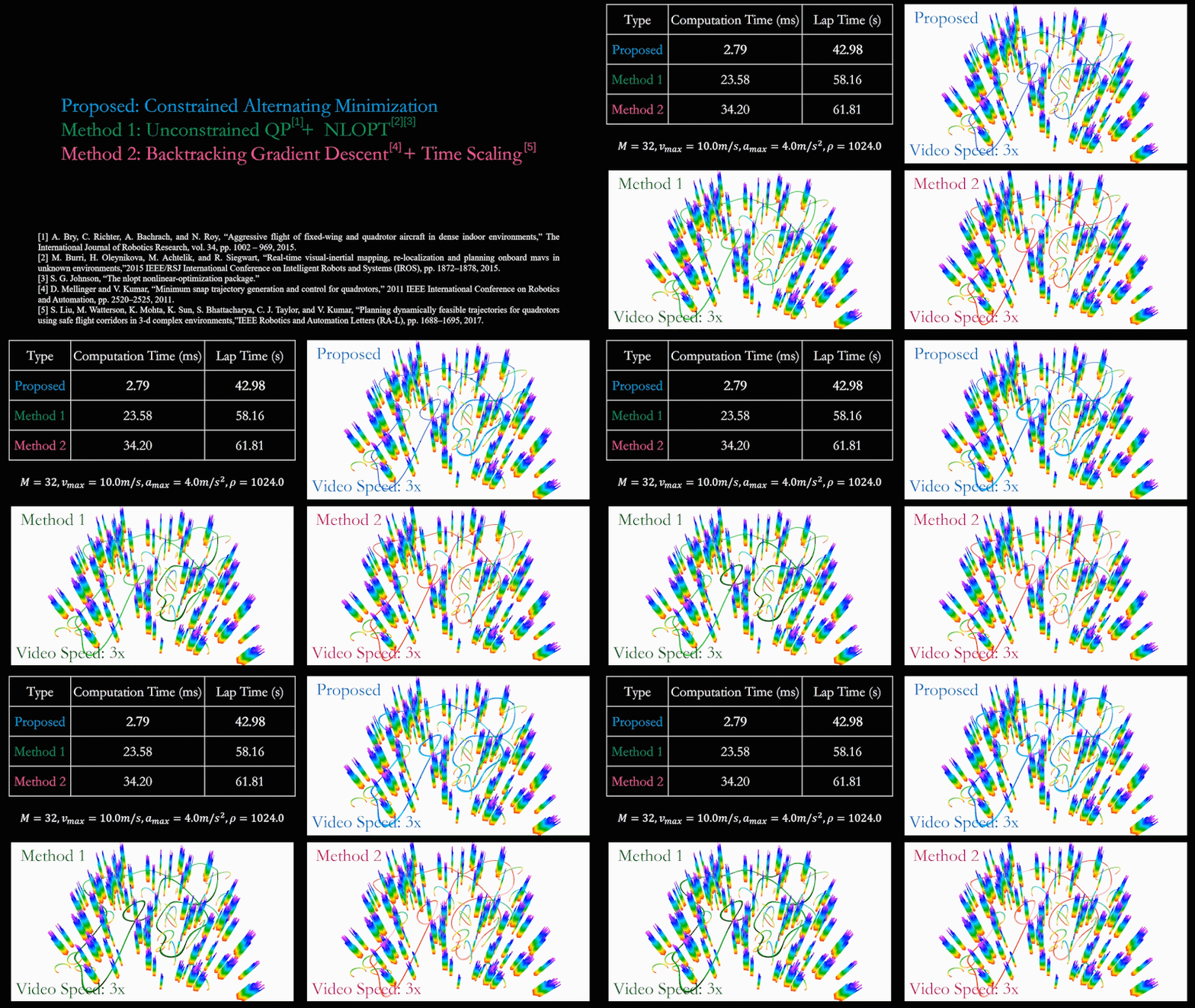
We compare our method with Richter's method with time allocation optimized by NLopt (QP + NLOPT) and Mellinger's method with durations properly scaled using Liu's method (BGD + Time Scaling). As is shown in the figure above, our optimizer has the fastest speed and the lowest cost when constraints are taken into consideration.
Two examples are provided in this repository.
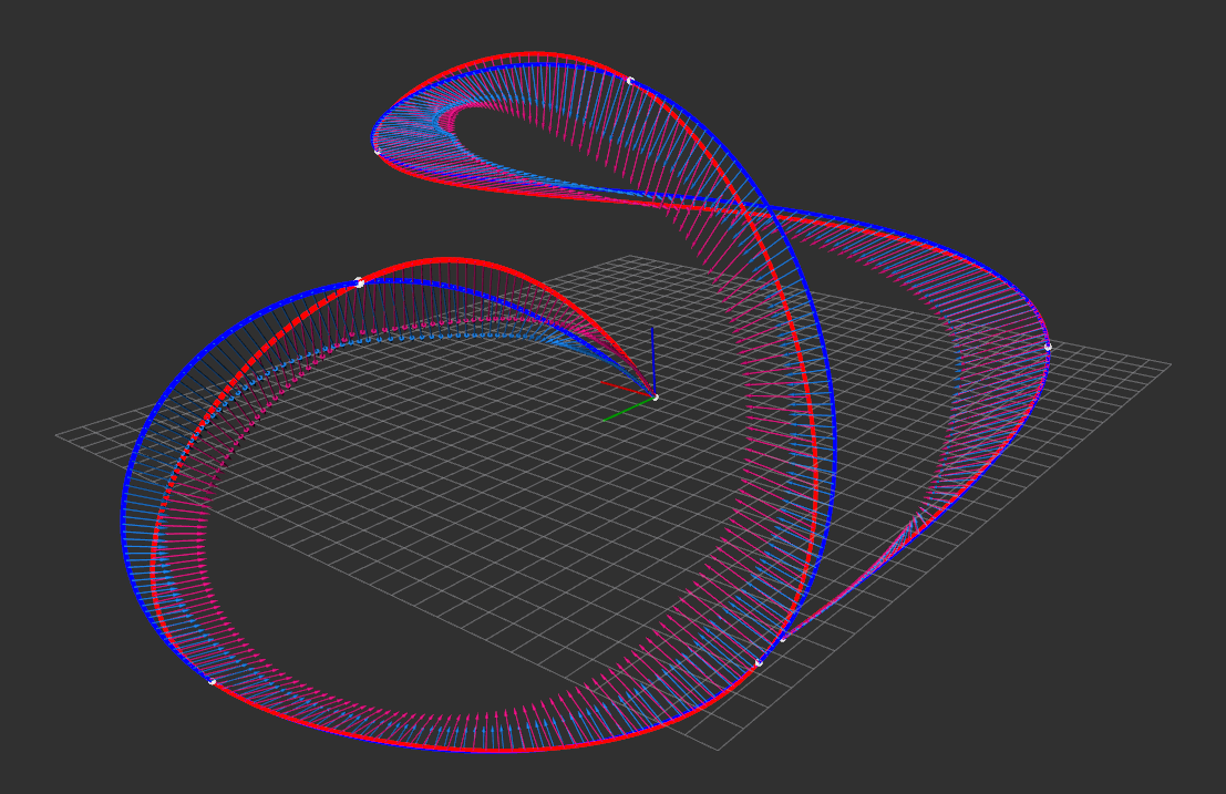
Example 0 contains a simple comparison between the constrained case of our method against conventional method which uses heuristic time allocation along with time scaling. The lap time, maximum velocity/acceleration rate, cost function value, and visualization are provided.
-
Building
To build this example, first make sure you have ROS properly installed. Desktop-full install is recommended. Second, clone this repository into the src directory of your ROS workspace. Rename it am_traj then move the example1 subdirectory to somewhere else, because we only consider the building of example0 here. Use the following command to install Eigen if they are not ready.
sudo apt install libeigen3-devNow cd into your current ROS workspace
catkin_make -
Running
source devel/setup.bash
rospack profile
roslaunch example0 example0.launch
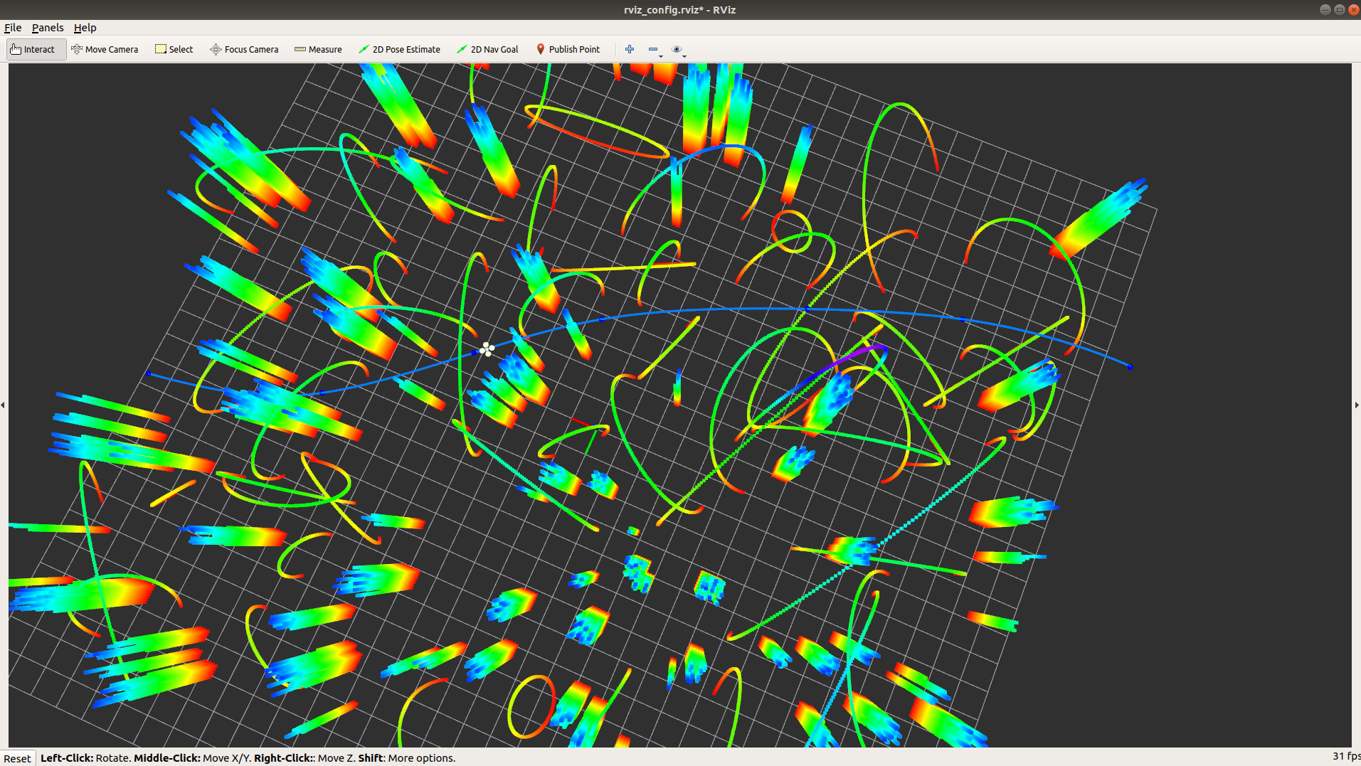
Now you can see the example 0 is running with visualization showing in rviz.
-
Parameters Setting
It is strongly recommended that modifying parameters after roughly going through our related papers. The parameters for objective should satisfy the corresponding assumption. For example, zero weight for time is illegal. Although our method is quite efficient when initial guess is far from optimum, it is still a first-order method with no Hessian info leveraged. Technically speaking, the best convergence rate for first-order method under smooth nonconvex consumption is sublinear, which means higher precision requires much more iterations. Therefore, we suggest that the relative tol should be set as 0.02~0.001. Pratically, time allocations [1.00, 2.00, 4.00, 0.30] and [1.01, 2.02, 4.04, 0.303] won't make much difference for real-time usage.
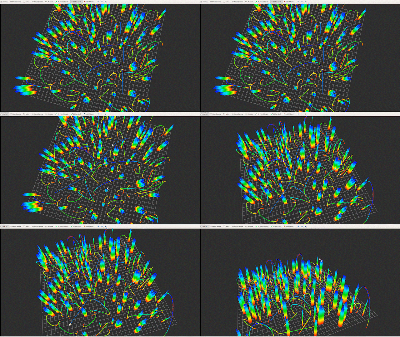
Example 1 contains a complete global planner simulation procedure. In this example, we adopt an RRT* based waypoints selector proposed by Richter et al.. Based on the selector, we use our library to generate a optimal feasible trajectory. The whole planner is able to do global traejctory generation in real time.
-
Building
To build this example, first make sure you have ROS and Eigen properly installed as described in previous example. Moreover, some parts of the simulation require GCC 7. Therefore, if your GCC version is below the required version, the following commands help you install it without changing your default compiler.
sudo apt-get install -y gcc-7 g++-7 && sleep 0.2;
sudo update-alternatives --install /usr/bin/gcc gcc /usr/bin/gcc-5 60 --slave /usr/bin/g++ g++ /usr/bin/g++-5 && sleep 0.2;
sudo update-alternatives --install /usr/bin/gcc gcc /usr/bin/gcc-7 50 --slave /usr/bin/g++ g++ /usr/bin/g++-7;
Second, use the following commands to install PyGame and OMPL.
sudo apt install python-pygame
cd ~/Desktop/
wget https://github.com/ompl/ompl/archive/1.4.2.zip
unzip 1.4.2.zip
cd ompl-1.4.2
mkdir build
cd build
cmake ..
make
sudo make install
Third, clone this repository into the src directory of your ROS workspace. Rename it am_traj. Now cd into your current ROS workspace.
catkin_make -
Running
Type following commands to start all nodes first.
source devel/setup.bash
rospack profile
roslaunch example1 example1.launch
Open a new terminal in your current ROS workspace and then
source devel/setup.bash
python src/am_traj/example1/key2joy.py
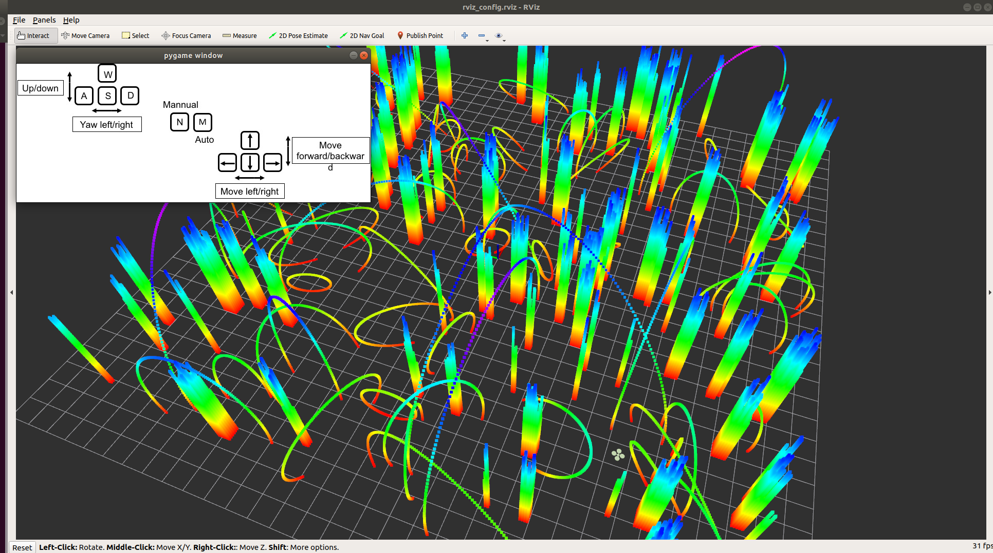
Now you can see an rviz window and a pygame window, which are shown below.
First, we should keep the pygame window active by click it once. Then, press N on your keyboard to activate manual mode. Press W/A/S/D and Up/Down/Left/Right on your keyboard to control the white quadrotor's height/yaw and horizontal movement respectively. Please navigate the quadrotor to a safe region. After that, press M on your keyboary to enter auto mode such that global planner is activated.
To navigate the quadrotor to any region safely, you should click once the following button on tools bar of rviz.
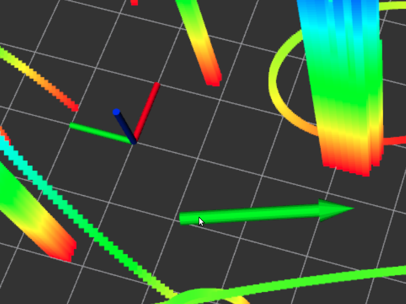
Once the button is clicked, you can move your mouse arrow to any free region you want. Click the place and hold it, then a green arrow appears as is shown in the following figure. You can change the direction of the green arrow. It is worth noting that, the angle between this arrow and positive part of x-axis (red axis) decides the relative height you want the quadrotor to keep at this region. The arrow in figure below gives 60 degrees which means the desired height is 60/180*MapHeight.
Now unhold the click, the global planner will finds you an appropriate trajectory instantly. The quadrotor then tracks the trajectory.
-
Conclusion
In most cases, the planner in this example is far faster than sampling-based kinodynamic planner, which may take several seconds to find an relative good trajectory for quadrotors. However, the RRT* used for waypoints selection can still take a relative long time (0.05 ~ 0.10 s) in comparison with our trajectory optimizer (about 0.5 ms for unconstrained case and 2.0 ms for constrained case). What's more, the waypoint selector does not consider the dynamics. That's to say, it is possible that wierd waypoints may be selected, when initial speed is large or obstacles are too dense. We claim that this is the inherent property of the adopted waypoint selector.
-
The library implements a specific order of polynomial trajectory optimization. If higher or lower order is required, it is recommended to refer to our related papers, where the framework used in the library are described and analyzed more flexibly.
-
The self-developed toolkit "root_finder.hpp" used in this library is an portable substitution to the suggested modern univariate polynomial real-roots solver in our related paper. It is more efficient in our scene than the wide used TOMS493: Jenkins–Traub Algorithm. For detailed performance, please refer to the corresponding repository. If efficiency is much more important to you, we suggest an closed-source solver RS-ANewDsc from Max Planck Institute for Informatics.
-
Currently, we only implement feasibilty checker for dynamic constraints. If only your constraints can be expressed in multivariate polynomial of trajectory or its higher derivatives. You can transform it into compatible format and utilize some functions in this library to accomplish simple yet solid check for it.
-
The library will support optimizing waypoints in the future, following the general framework in our paper. However, the spatial constraints depend on specific planning method. Therefore, feel free to modify all codes in the library if you need to optimize waypoints.
-
Thanks Helen Oleynikova et al. a lot for their open-source project. In our benchmark, some modules in compared methods are modified from their projects.
The source code is released under GPLv3 license.
For any technical issues, please contact Zhepei WANG (wangzhepei@live.com) or Fei GAO (fgaoaa@zju.edu.cn).
For commercial inquiries, please contact Fei GAO (fgaoaa@zju.edu.cn).
