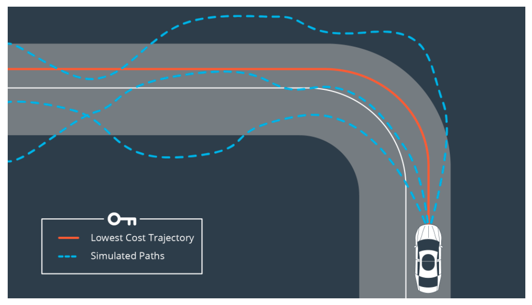
In this Udacity Self-driving-car engineer nanodegree project the goal was to apply model predictive control (MPC) to control a car around a race track, essentially controlling the steering and throttle (acceleration). In MPC the control problem is modeled as an optimization problem using the kinematics or dynamics model of the car as contraints for the kinematics parameters and physical limits such as maximum steering angle and acceleration/deceleration as bounds for our control input parameters steering and throttle. The optimizer is calculating a whole trajectory in each iteration and eventually chooses the one with the lowest cost. Every point on that trajectory consists with a vehicle kinematic state and control input / actuator values. Only the actuator value pair of the first point on the final trajectory is used as control input. Because the project aims to be somewhat realistic there is an actuation latency of 100ms which has to be incorporated in the trajectory prediction.
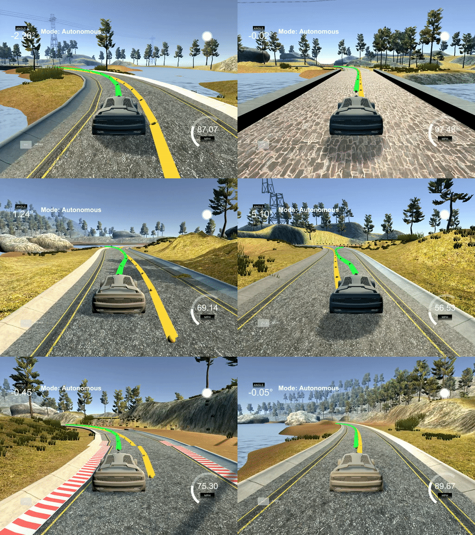
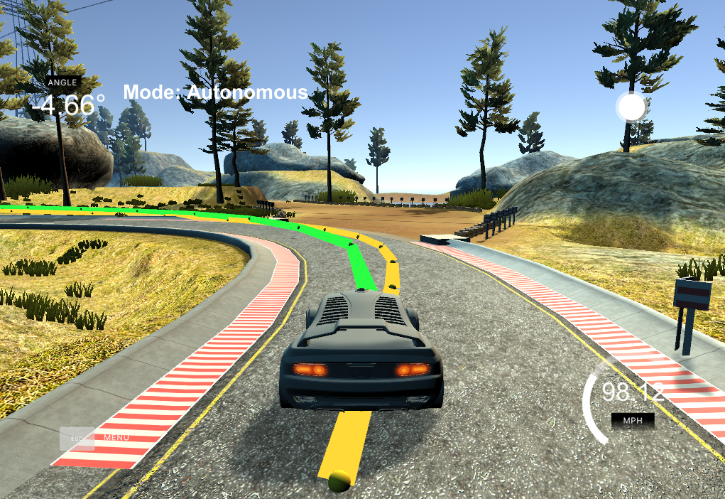
The following screenshot of the simulator shows the MPC path displayed in green and the reference path in yellow. Those paths are fitted polynomials to the waypoints which appear as small spheres along the path.
The data structures which are used for communication with the simulator are documented in DATA.md.
A simulator provides the following state variables as telemetry messages:
- X and Y Position of the car in a global map coordinate system
- Heading / yaw angle
- Lateral velocity
- A list of waypoints in X and Y in a global map coordinate system
By fitting a polynomial to the given waypoints we get a function that resembles the curve of the road ahead. Usually a 3rd degree polynomial can be a good estimate of most road curves. Before fitting the waypoints to the polynomial function we have to transform the global map coordinates into the local vehicle coordinate frame.
- List of reference trajectory waypoints in vehicle coordinate frame for visualization
- List of predicted waypoints by MPC in vehicle coordinate frame for visualization
- Control inputs: steering angle in rad [-25°, +25°], throttle [-1, +1]
For this project a Constant Steering Angle and Velocity (CSAV) kinematic bicycle model is assumed, in which the correlation between v and the turn-rate omega can be modeled by using the steering angle as constant variable and derive the yaw rate from v, the steering angle and a constant Lf which describes the length from the front of vehicle to its center-of-gravity.
That means our system states consists of:
- Position X and Y in an global map coordinate system (
pxandpy) - Heading / yaw angle (
psi) - Lateral velocity (
v) - Yaw rate, derived from steering angle and
v((v / Lf) * steer_angle) - Cross track error (
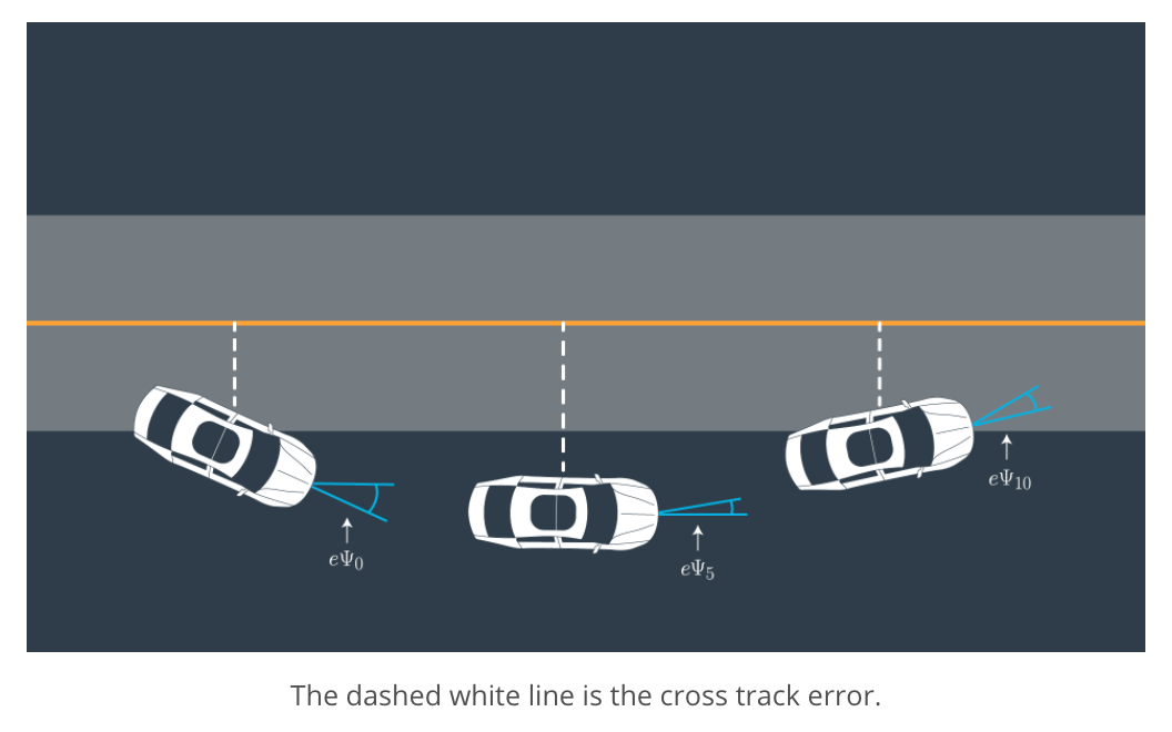
cte) - error between desired and the actual position. - Orientation Error (
epsi) - difference between our desired heading and actual heading.
The cross track error and orientation error (epsi) are illustrated in the following figure:

Once we fitted a polynomial function across the reference waypoints we can use it to calculate the errors cte and epsi.
The cross track error is caluclated by just evaluating the polynomial function at 0, whereas the heading angle error is the arctan of the derivative of the polynomial function, also evaluated at 0.
So to summarize:
- cte = f(0)
- epsi = argctan(f'(0))
The following kinematics equations are used for setting up the constraints in the optimizer as well as for future state prediction to compensate actuator latency:
px1   = px0   + v0 * dt * cos(psi0)
py1   = py0   + v0 * dt * sin(psi0)
psi1  = psi0  + v0 / Lf * steer_angle * dt
v1    = v0    + throttle * dt
Lfis the length from front of vehicle to its center-of-gravity, a parameters which has been calculated and provided Udacity (Lf = 2.67).- Car acceleration
throttlewill be between -1 (full brake) and +1 (full acceleration). - Car steering angle
steer_anglewill be between -25° and +25°.
We can also predict the next cte and epsi based on our actuations:
cte1  = cte0   - v0 * sin(epsi0) * dt
epsi1 = epsi0  + v0 / Lf * steer_angle * dt
Different trajectories are calculated over the prediction horizon by the optimizer, the horizon is the duration over which future predictions are made. We’ll refer to this as time T.
Tis the product of two other variables,Nanddt.Nis the number of timesteps in the horizon.dtis how much time elapses between actuations.
For example, if N were 20 and dt were 0.5, then T would be 10 seconds.
N and dt are hyperparameters which need to be tuned. But in general T should be as large as possible, while dt should be as small as possible.
Because of the actuation latency of 0.1 I also set dt also to 0.1. It makes sense because due to the delay the timing grid at which the optimizer will get invoked will be at multiples of 0.1s anyway. Predicting trajectories with time steps smaller than this delay leads to shaky behaviour.
As for the number of timesteps N I stuck with the default value of 10, which just gave good results even at higher speeds like 100mph, so the prediction horizon was long enough for safe driving.
The trajectory with the lowest cost will be chosen by the optimizer, that means that the cost function has to be designed carefully.
A cost function should contain all independed control variables which are actively changed by the optimizer.
Those variables can be taken directly or more complicated terms can be formulated such as derivatives of those variables.
Then a weight for each of those terms is assigned in order to able to give some terms a higher importance than others.
Eventually those terms are squared (L2² norm) and added up to a scalar sum.
Taking into consideration that our primary objective is to minimize cte and epsi those weights should be the highest.
Increasing also the weights for consecutive steering angles and the change in steering angles helps getting a very smooth path.
The least of our concerns is going as fast as possible, that's why I didn't change those weights.
So in my approach I focussed only on penalizing steering actuations and the gaps between sequential actuations because it gave the best and smoothest results.
Because the weight for the cross track error term should be in a similar range it got the same weight steering_cost_weight.
  for (int t = 0; t < N; t++) {
    fg[0] += steering_cost_weight * CppAD::pow(vars[cte_start + t], 2);
    fg[0] += CppAD::pow(vars[epsi_start + t], 2);
    fg[0] += CppAD::pow(vars[v_start + t] - ref_v, 2);
  }

  // Minimize the use of actuators, for all sampling points except last one (N-1).
  for (int t = 0; t < N - 1; t++) {
    fg[0] += steering_cost_weight * CppAD::pow(vars[delta_start + t], 2);
    fg[0] += CppAD::pow(vars[a_start + t], 2);
  }

  // Minimize the value gap (derivative) between sequential actuations,
  // for all sampling points except the last two (N-2).
  for (int t = 0; t < N - 2; t++) {
    fg[0] += steering_cost_weight * CppAD::pow((vars[delta_start + t + 1] - vars[delta_start + t]), 2);
    fg[0] += CppAD::pow(vars[a_start + t + 1] - vars[a_start + t], 2);
  }
For determining steering_cost_weight I used a heuristic that says that on straight roads (low curvature, high radius) the steering penalty should be relaxed and in narrow curves (high curvature, low radius) steering should get the main focus for the optimizer by setting a high weight, see here:
  const double max_radius = 1e3;
  // Calculate radius and catch division by zero
  if (fabs(coeffs[2]) > std::numeric_limits<double>::epsilon()) {
      // y(x)   = a*x^3 + b*x^2 + c*x + d
      // y'(x)  = 3*a*x^2 + 2*b*x + c,    y''(x) = 6*a*x + 2*b
      // coeffs = [d, c, b, a]
      // R(x)   = ((1 + f'(x)^2)^1.5) / abs(f''(x))
      //        = ((1 + (3*a*x^2 + 2*b*x +c)^2)^1.5 / abs(6*a*x+2*b)
      // R(0)   = ((1 + c^2)^1.5 / abs(2*b)
      radius = pow(1.0 + pow(coeffs[1], 2), 1.5) / fabs(2.*coeffs[2]);
      if (radius > max_radius)
        radius = max_radius;
  } else {
      radius = max_radius;
  }

  avg_radius(radius);
  steering_cost_weight = steering_smoothness * (max_radius / avg_radius);
The hyper parameter steering_smoothness was eventually set to 200.
The issue with latency in a control system like a car is that by the time the car executes the next actuator commands the state has changed from the previously calculated one already and is not reflecting the current situation anymore. This can lead to instability like oscillations in a control system.
Dealing with actuator latency means compensating that effect by estimating the latency and modelling it the kinematic model which is used for state estimation and prediction such as given below:
px    += v * cos(psi) * latency_s
py    += v * sin(psi) * latency_s
psi   += v * steer_angle / Lf * latency_s
cte   += v * sin(epsi) * latency_s
epsi  += v * steer_angle / Lf * latency_s
v     += throttle * latency_s
In this project there are two places where this can be done:
- Directly when we received back the telemetry data from the simulator before calculating the polynomial function parameters (coefficients).
- After calculating the polynomial coefficients for the reference trajectory, just before the current state is given to the optimizer to find the next actuation values.
After some testing it seems that the latter option leads to a more robust behaviour, because due to some inaccuracies in the estimated latency the reference path starts to shake and therefore also the MPC generated trajectory, which leads to severe oscillations and eventually to a crash. There is one thing I did not figure out though, the latency value which worked best was around 0.065s although the program enforces a delay of 0.1s and the optimizer causes another 0.02 to 0.03 seconds delay which should add up to around 0.13s which would need to be compensated. It even depends which detail mode you select in the simulator, a higher amount of details leads to a higher delay. Compensating only for 0.065s did work best graphics quality mode "good", getter lower or higher with the anticipated delay made the controller unstable. In graphics quality mode "fantastic" it seems that 0.1s work better.
In the end I was able to successfully drive around the test track with v_ref set to 110mph and an estimated average velocity of around 80mph for half and hour, without any crashes or incidents.
-
cmake >= 3.5
-
All OSes: click here for installation instructions
-
make >= 4.1(mac, linux), 3.81(Windows)
- Linux: make is installed by default on most Linux distros
- Mac: install Xcode command line tools to get make
- Windows: Click here for installation instructions
-
gcc/g++ >= 5.4
- Linux: gcc / g++ is installed by default on most Linux distros
- Mac: same deal as make - [install Xcode command line tools]((https://developer.apple.com/xcode/features/)
- Windows: recommend using MinGW
-
- Run either
install-mac.shorinstall-ubuntu.sh. - If you install from source, checkout to commit
e94b6e1, i.e.Some function signatures have changed in v0.14.x. See this PR for more details.git clone https://github.com/uWebSockets/uWebSockets cd uWebSockets git checkout e94b6e1
- Run either
-
Ipopt and CppAD: Please refer to this document for installation instructions.
-
Simulator. You can download these from the releases tab.
-
Not a dependency but read the DATA.md for a description of the data sent back from the simulator.
- Clone this repo.
- Make a build directory:
mkdir build && cd build - Compile:
cmake .. && make - Run it:
./mpc.
- It's recommended to test the MPC on basic examples to see if your implementation behaves as desired. One possible example is the vehicle starting offset of a straight line (reference). If the MPC implementation is correct, after some number of timesteps (not too many) it should find and track the reference line.
- The
lake_track_waypoints.csvfile has the waypoints of the lake track. You could use this to fit polynomials and points and see of how well your model tracks curve. NOTE: This file might be not completely in sync with the simulator so your solution should NOT depend on it. - For visualization this C++ matplotlib wrapper could be helpful.)
- Tips for setting up your environment are available here
- VM Latency: Some students have reported differences in behavior using VM's ostensibly a result of latency. Please let us know if issues arise as a result of a VM environment.
We've purposefully kept editor configuration files out of this repo in order to keep it as simple and environment agnostic as possible. However, we recommend using the following settings:
- indent using spaces
- set tab width to 2 spaces (keeps the matrices in source code aligned)


