This repository contains all the code for a localization software for autonomous vehicles. The initial location can be a noisy GPS estimate. For more precise localization lots of (noisy) sensor and control data can be used. Both the initial location and the sensor and control data are simulated/provided by a simulator while running the code (see below in the section Running the Code.
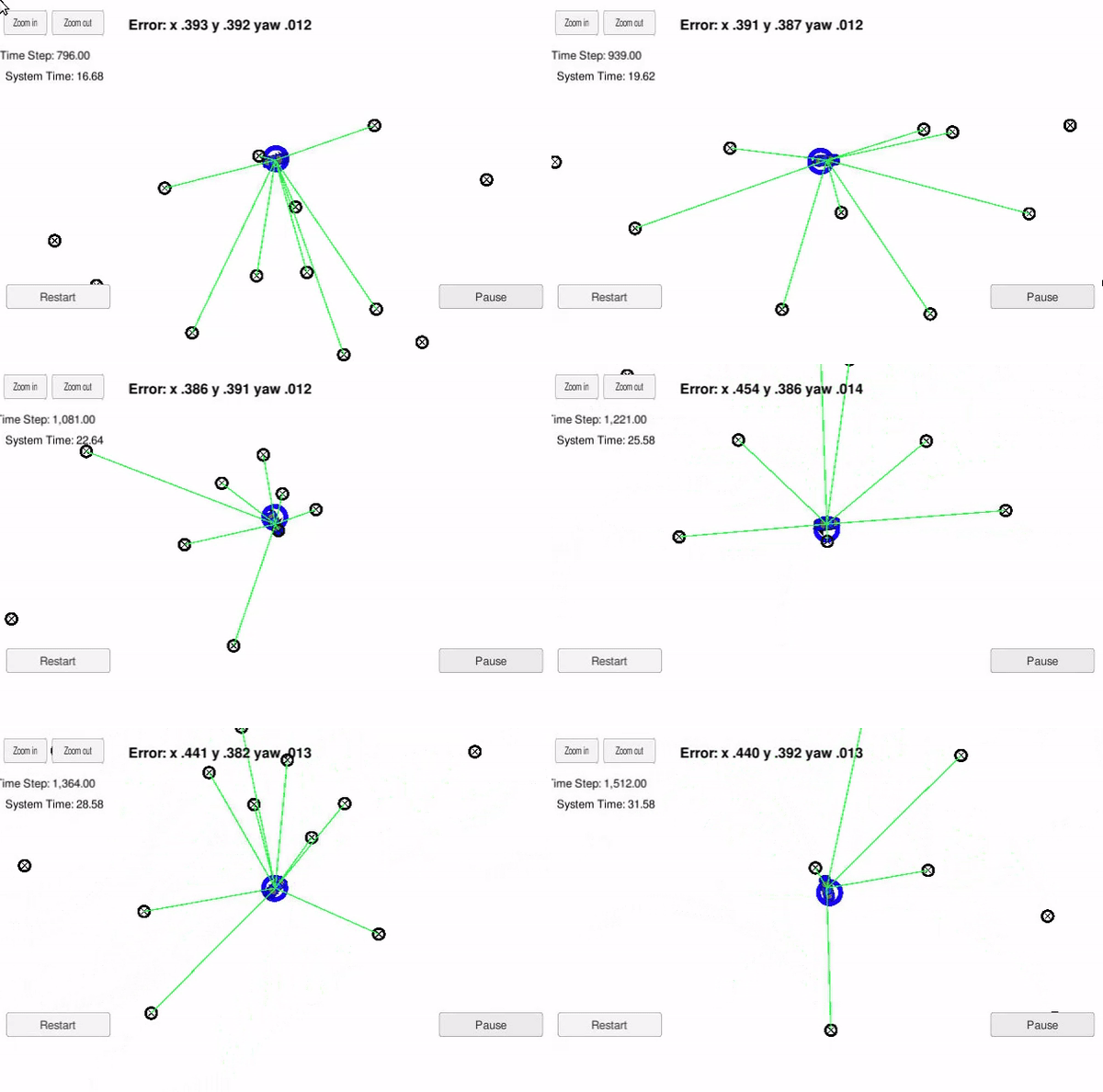
For validation of the software, a simulator is used. This can be seen like a vehicle that is kidnapped inside a closed environment and has no idea of its location. The vehicle drives through the environment and takes roughly 2400 steps with change in orientation and position. The location of the vehicle is predicted using a 2-dimensional Particle Filter implemented in C++.
The particle filter will be given a map and some initial localization information (analogous to what a GPS would provide). At each time step the filter will also get observation and control data.
Localization in terms of autonomous vehicles means to predict the position with a high accuracy in the range of 3-10 cm. This location is in reference to a global map in which the vehicle is stationary or moving.
One simple way to localize a vehicle is to use data from GPS, which uses triangulation to predict the position of an object. But GPS doesn't always provide high accuracy. In case of a strong GPS signal, the accuracy in location could be in the range of 1-3 m whereas in the case of a weak GPS signal, the accuracy drops to a range of 10-50 m. Hence the use of only GPS is not reliable.
To achieve an accuracy of 3-10 cm, sensor information from various sensors such as Laser sensors (LIDAR), Radial distance and angle sensor (RADAR) are fused together using a Particle Filter.
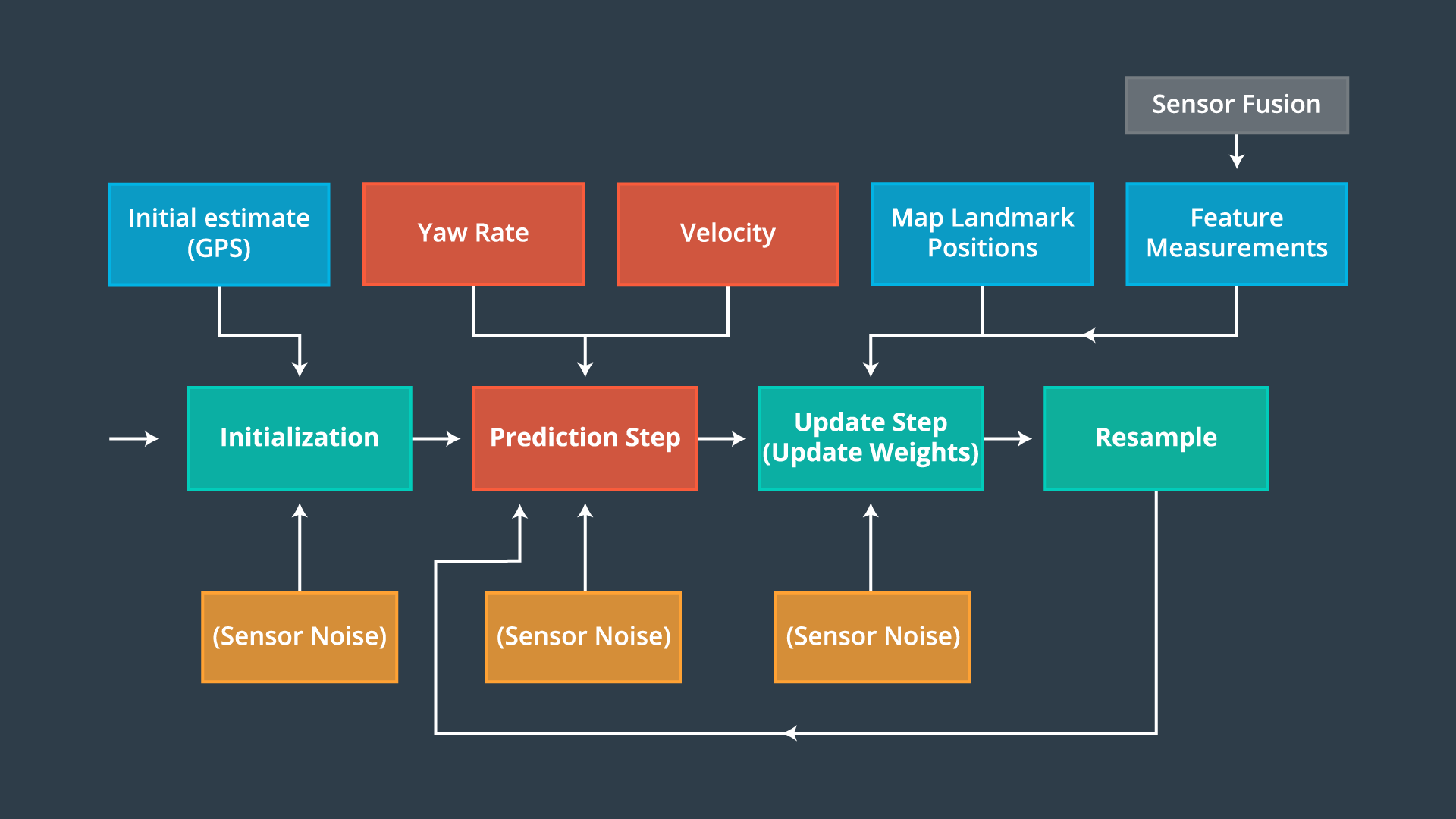
An overview of the algorithm is illustrated in the following diagram:

The C++ program for localization was implemented using the following major steps:
- The number of particles are defined (num_particles = 100).
- All particles are initialized using GPS measurements with mean equal to the location received from GPS and standard deviation equal to the GPS measurement uncertainty (both provided by the simulator).
- Initial weight of all particles is set to one (particle.weight = 1.0).
- The location of each particle at the next time step after the time 'delta_t' is predicted using the following formulae. The calculation depends on whether the yaw rate equals 0 or not):

- The vehicle uses LIDAR to sense its distance to landmarks (observation measurements). This is received as a list of x, y coordinates along with measurement noise mapped as standard deviation in x and y. Since the LIDAR sensor is installed on the vehicle, these observations are received in x, y coordinates relative to the motion direction of the vehicle.
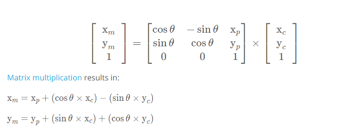
- These observation measurements are transformed from vehicle coordinates (local coordinate system) to map coordinates (global coordinate system) using the following homogenous transformation matrix.
-
For every observation (x, y) the nearest landmark is taken (nearest neighbour) associated to this observation. This is done by finding the landmark with the lowest difference/euclidean distance. Each landmark has an actual, real, known position (x, y). Each observation is exactly such a position in global coordinates (after transformation). A certain measurement is expected for a certain landmark, namely exactly in such a way that the observation (transformed into global coordinates) corresponds exactly to the landmark - the deviation is therefore zero. This would be the ideal observation, hence you would have found the perfect fitting particle with its position that would be exacty the vehicle's position. Since the world is not ideal and your algorithm probably will not take the best particle immediately, the algorithm has to find the best particle. This is why it is called particle filter. The algorithm now performs all these calculations for all particles and finally returns the best fitting particle. This is the particle where the difference between its coordinates and the observation coordinates is the smallest.
-
If you combine the particle's position with an observation, you land at some place. From this place you look for the nearest landmark and associate this landmark to the observation. There is a gap/deviation/difference from this measured location and the actual, real location of the landmark you would expect. This deviation results in the so-called multivariate gaussian probability (calculation see below). The lower the gap is, the higher the calculated probability will be. The weight of a particle is the measure of how close the particle is to the ground truth of the vehicle. The higher the weight, the more accurate is the particle's prediction.
-
For each observation the multivariate Gaussian normal distribution with its closest landmark is calculated and all resulting probabilities are multiplied. The result is the particle weight.
Multivariate Gaussian probability:

- All of the above has related to one single particle. Now the calculations are carried out for each individual particle. The particles with the highest weights (i.e. the smallest deviations in relation to the observations and landmarks) gradually prevail in the algorithm (filtering). Hence, at the end of each weight update step, 'resampling' of particles with replacement is done to remove highly improbable particles.
-
Resampling involves retaining of particles with higher weight and crushing of particles with lower weight. Once resampling is done, the particle with highest weight is chosen. This particle gives most accurate prediction of vehicle's location.
-
The location provided by particle with highest weight is then compared with the ground truth and error in the system is calculated.
The simulator can be downloaded here
This repository includes two files that can be used to set up and install uWebSocketIO for either Linux or Mac systems. For windows you can use either Docker, VMware, or even Windows 10 Bash on Ubuntu to install uWebSocketIO.
Once the install for uWebSocketIO is complete, the main program can be built and ran by doing the following from the project top directory.
- mkdir build
- cd build
- cmake ..
- make
- ./particle_filter
Alternatively some scripts have been included to streamline this process, these can be leveraged by executing the following in the top directory of the project:
- ./clean.sh
- ./build.sh
- ./run.sh
Here is the main protocol that main.cpp uses for uWebSocketIO in communicating with the simulator.
INPUT: values provided by the simulator to the c++ program
// sense noisy position data from the simulator
["sense_x"]
["sense_y"]
["sense_theta"]
// get the previous velocity and yaw rate to predict the particle's transitioned state
["previous_velocity"]
["previous_yawrate"]
// receive noisy observation data from the simulator, in a respective list of x/y values
["sense_observations_x"]
["sense_observations_y"]
OUTPUT: values provided by the c++ program to the simulator
// best particle values used for calculating the error evaluation
["best_particle_x"]
["best_particle_y"]
["best_particle_theta"]
//Optional message data used for debugging particle's sensing and associations
// for respective (x,y) sensed positions ID label
["best_particle_associations"]
// for respective (x,y) sensed positions
["best_particle_sense_x"] <= list of sensed x positions
["best_particle_sense_y"] <= list of sensed y positions
The directory structure of this repository is as follows:
root
|   build.sh
|   clean.sh
|   CMakeLists.txt
|   README.md
|   run.sh
|
|___data
|   |
|   |   map_data.txt
|
|
|___src
    |   helper_functions.h
    |   main.cpp
    |   map.h
    |   particle_filter.cpp
    |   particle_filter.h
The file particle_filter.cpp contains the framework of a ParticleFilter class and some associated methods. Read through the code, the comments, and the header file particle_filter.h to get a sense for what this code is expected to do.
The file src/main.cpp will actually be running the particle filter and calling the associated methods.
You can find the inputs to the particle filter in the data directory.
map_data.txt includes the position of landmarks (in meters) on an arbitrary Cartesian coordinate system. Each row has three columns
- x position
- y position
- landmark id
- Map data provided by 3D Mapping Solutions GmbH.

