- Abstract
- Background
- Introduction
- Selecting the Robot
- Building the Robot
- World: the provided world
- World: creating a new world
- Creating the launch files
- Robot, map the world
- Results
- Discussion
- Future work
The target of this project is to create a 2D occupancy grid and 3D octomap from a provided simulated environment. Furthermore, create a simulated environment (world) to be mapped as well.
The RTAB-Map framework is used to allow the robot to map the environment in 3D. Also, Gazebo and ROS are used for simulation.
In robotic mapping and navigation, the simultaneous localization and mapping (SLAM) is the computational problem of constructing or updating a map of an unknown environment while simultaneously keeping track of an agent's location within it. We need a map to localize and we need to localize to make the map.
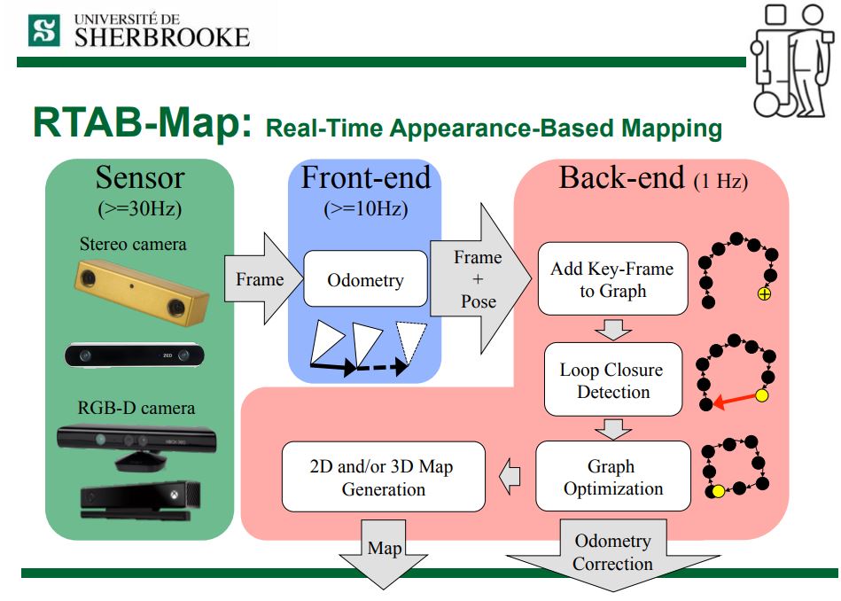
Fig. 2 - Workflow how RTAB-Map works.
RTAB-Map (Real-Time Appearance-Based Mapping) is a RGB-D Graph-Based SLAM approach based on an incremental appearance-based loop closure detector. The loop closure detector uses a bag-of-words approach to determinate how likely a new image comes from a previous location or a new location. When a loop closure hypothesis is accepted, a new constraint is added to the map’s graph, then a graph optimizer minimizes the errors in the map. A memory management approach is used to limit the number of locations used for loop closure detection and graph optimization, so that real-time constraints on large-scale environnements are always respected. In this project a robot is equiped with Kinect and RTAB-Map to generate 6DoF RGB-D mapping.
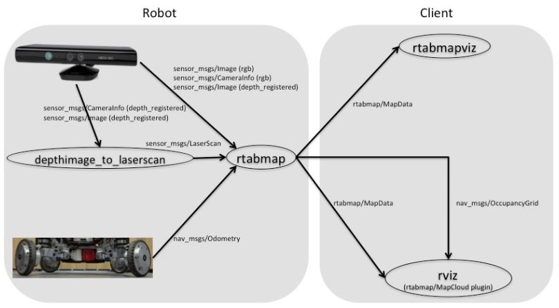
This project uses rtabmap_ros that is a wrapper of RTAB-Map to provide the mapping functionalities used by the robot to map the environment. This package can be used to generate a 3D point clouds of the environment and/or to create a 2D occupancy grid map for navigation.
For image capture the project uses a Kinect camera (RGB-D) and, to make the Kinect publish in the scan topic, the project uses the following configuration.
Note that the configuration provides a method of mapping the depth point cloud into a usable scan topic that can be managed by RTAB-Map.
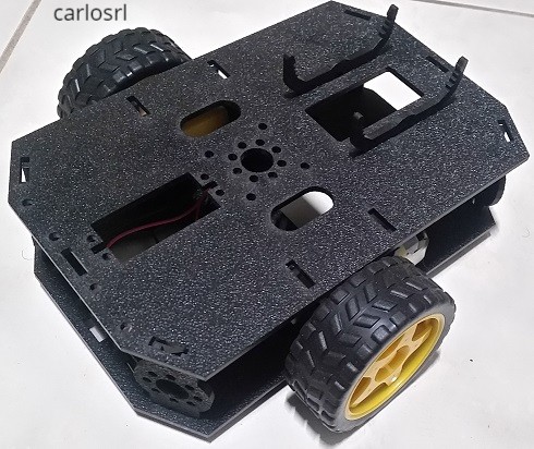
The target of this step is to chose a robot type, build the urdf model, load it into Gazebo and run the robot simulation to map the environment using the rtabmap-ros package. So, why not get a real robot to use as reference in the sumulation? Then we can apply the lessons learned in the real model. That sounds good. So, the figure below show the model selected.
Fig. 4 - Robot select as reference.
It is a two differential whelled robot using two step motors. So, adding more hardware components we can use it for mapping.
The urdf model must have:
- chassis
- right wheel
- left wheel
- caster
- RGB-D camera
- RGB camera
- laser scan
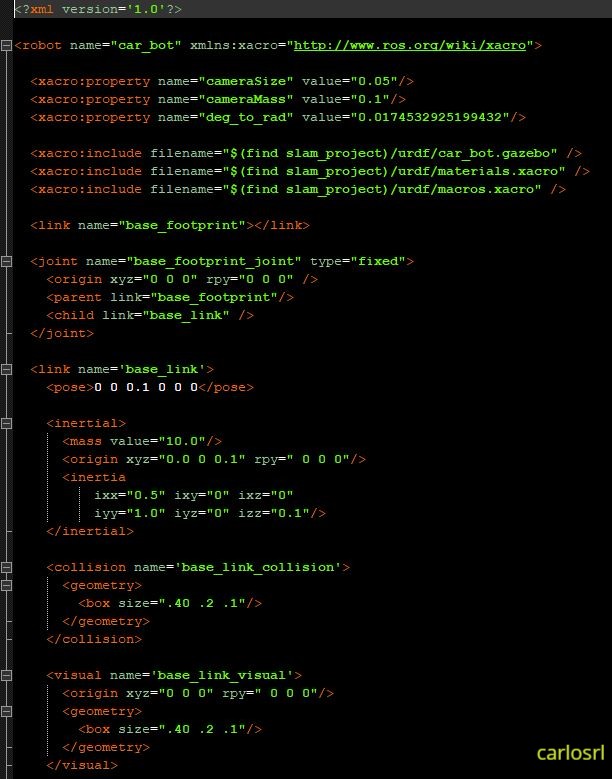
Based on the list above, two files were created: car_bot.xacro and car_bot.gazebo. The car_bot.xacro contain the urdf model definition and car_bot.gazebo contain the urdf sensor definition. The Fig. 5 shows part of the car_bot.xacro.
Fig. 5 - Part of robot URDF model.
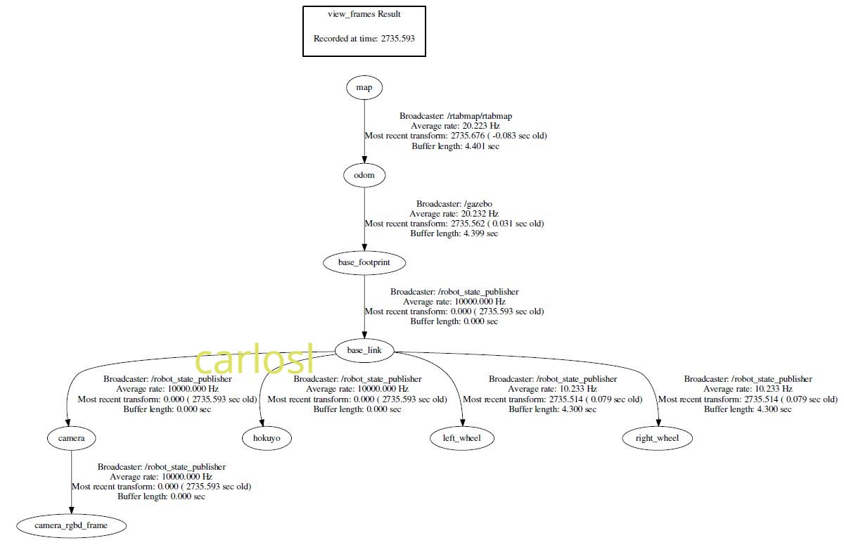
To see the final urdf model we can take a look the picture of frames in Fig. 6 that shows the robot model has a camera and a rgbd frames.
Fig. 6 - Robot frames.
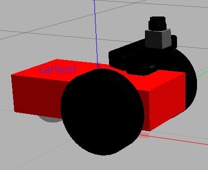
Using xacro elements and macros in xacro file, we can contruct the entire urdf model and load it into Gazebo tool. The result is in Fig. 7.
Fig. 7 - The robot model spawned in Gazebo tool.
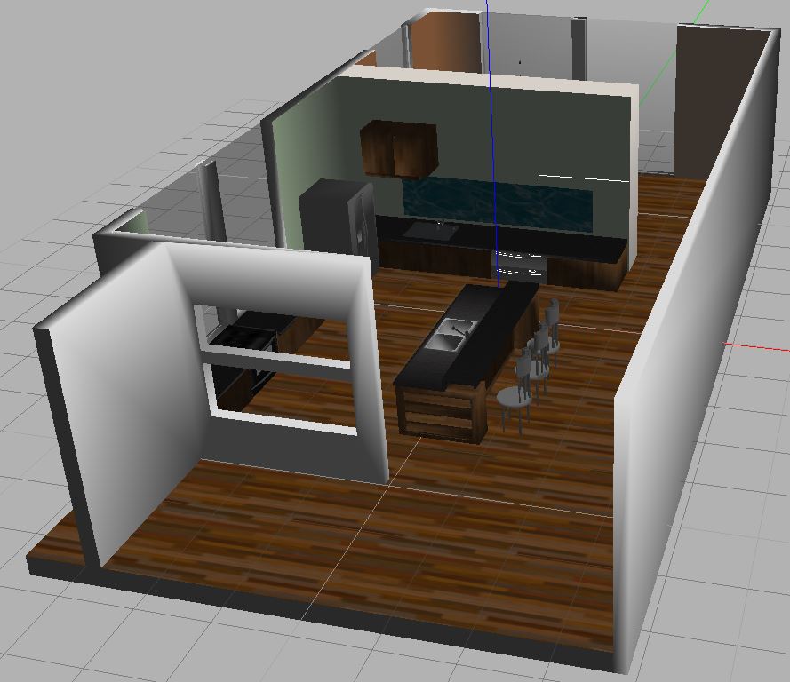
As the project title states, the project target is to map the world. So we have two worlds to be managed: the provided world and a new one that must be createded. The Fig. 8 shows the provided kitchen dining world.
Fig. 8 - The kitchen dining world
Note that the environment has a lot of features which will demand a heavy hardware resource in the mapping process.
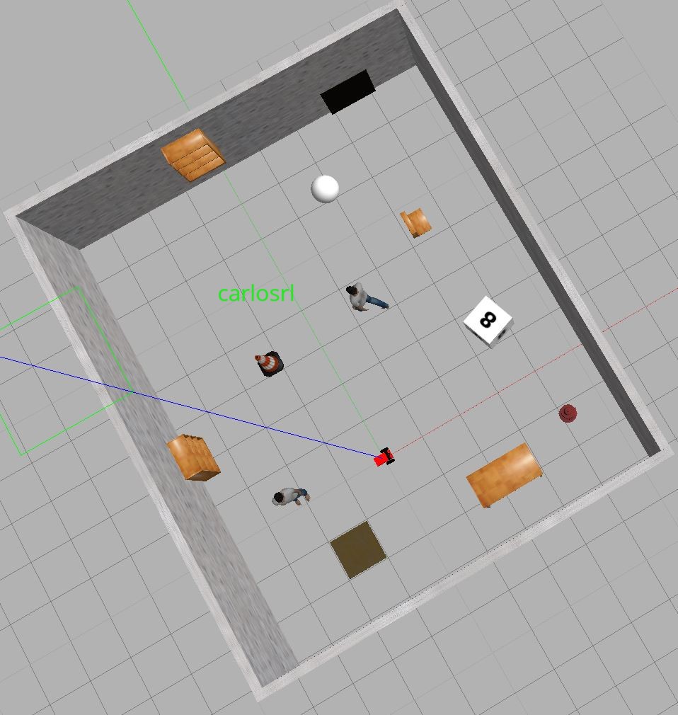
To create a new world we can use the Build Editor option in Gazebo tool. In the editor we can use existing objects and models or create new objects using the features provided in the editor tool. So, using walls, tables and others objects, we created a new world as showed in Fig. 9.
Fig. 9 - The new created world
At this point we have the robot model and the world environments. To manage the mapping process we need load the robot model, the world, launch the Gazebo simulation, launch the rtabmap-ros package and a teleop script to teleoperate the robot in the environment to allow it gather as much features, from the world, as possible.
To make the things easier, we can automate these steps creating launch files that will contain a set of commands that are executed using the roslaunch tool.
For illustration, the following snippet code is the world.launch content.
<?xml version="1.0"?>
<launch>
  <arg name="world" default="empty"/>
  <arg name="paused" default="false"/>
  <arg name="use_sim_time" default="true"/>
  <arg name="gui" default="true"/>
  <arg name="headless" default="false"/>
  <arg name="debug" default="false"/>

<!-- We resume the logic in empty_world.launch, changing only the name of the world to be launched -->
  <include file="$(find gazebo_ros)/launch/empty_world.launch">
    <!-- <arg name="world_name" value="$(find slam_project)/worlds/kitchen_dining.world"/> -->
    <arg name="world_name" value="$(find slam_project)/worlds/user_created.world"/>
    <arg name="paused" value="$(arg paused)"/>
    <arg name="use_sim_time" value="$(arg use_sim_time)"/>
    <arg name="gui" value="$(arg gui)"/>
    <arg name="headless" value="$(arg headless)"/>
    <arg name="debug" value="$(arg debug)"/>
  </include>

  <!-- spawn a robot in gazebo world -->
  <include file="$(find slam_project)/launch/car_bot_description.launch"/>

  <node name="car_bot_spawner" pkg="gazebo_ros" type="spawn_model" respawn="false" output="screen"
   args="-urdf -param robot_description -model car_bot"/>
</launch>
The launch file has the xml format as showed above. Note that world.launch file contain two wolds that are commented/uncommented depending on which world must be launched.
In addition to world.launch, we have the mapping.launch, used to load the rtabmap-ros package and the rtabmapviz or rviz, depending on the selection in the command line and the rviz.launch, used to load the rviz tool. Instead of rviz.launch, a different solution could be add the rviz command inside the mapping.launch and select it in command line.
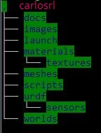
The final directory structure is showed in Fig. 10.
Fig. 10 - Directory structure
Putting all together, we can now start the mapping process.
Start launching the world and the robot model using the command
roslaunch slam_project world.launchNow launch the rtabmap with rtabmaprviz tool, using the command
roslaunch slam_project mapping.launchFinally, launch the teleop script to control the robot using the command
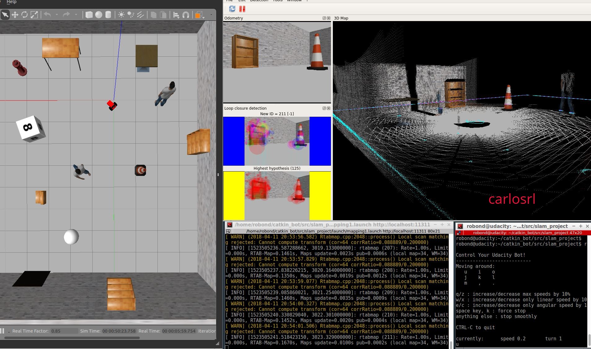
rosrun slam_project teleopMapping the created environment can be seen in Fig. 11
Fig. 11 - Robot mapping the user created world.
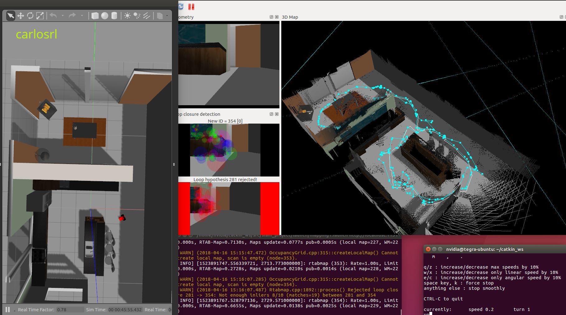
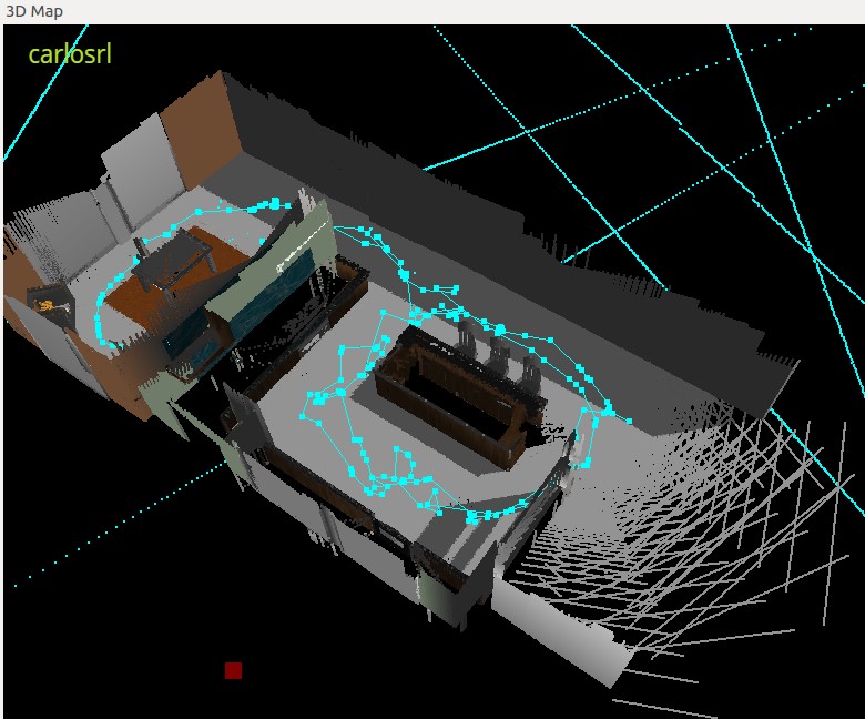
Mapping the provided environment can be seen in Fig. 12
Fig. 12 - Robot mapping the provided world.
While the robot is moving in the environment, in RTAB-Map we can see in realtime many features being collected like loop closure, feature mathing and so on.
In RTAB-Map loop closure is detected using a bag-of-words approach, that is commonly used in vision-based mapping. In RTAB-Map the default method for extracting features from an image is called Speeded Up Robust Features of SURF.
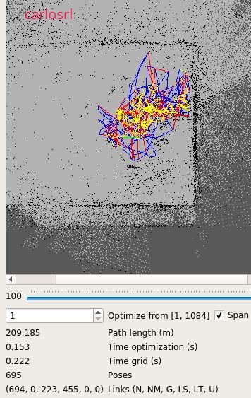
Fig. 13 - 2D image with no optimization for user created env.
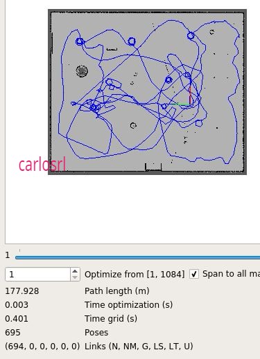
Fig. 14 - 2D image with optimization for user created env.
Note that global and local closure loop values are zeroed when optimization is applied.
For the provided environment, where we have more features, the 2D map is more clean as we can see in Fig. 15 and 16. Besides, we see few difference between optmized and no optimized 2D graphic.
Fig. 15. - 2D image with no optimization for provided env.
Fig. 16. - 2D image with optimization for provided env.
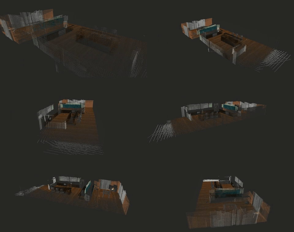
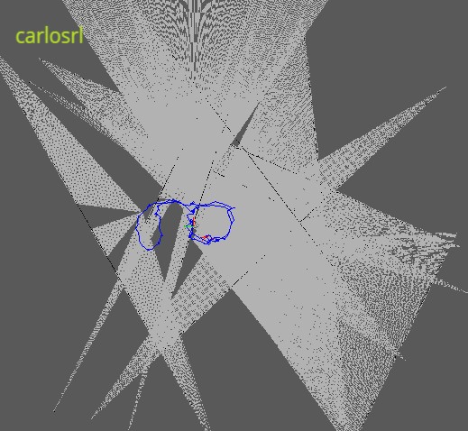
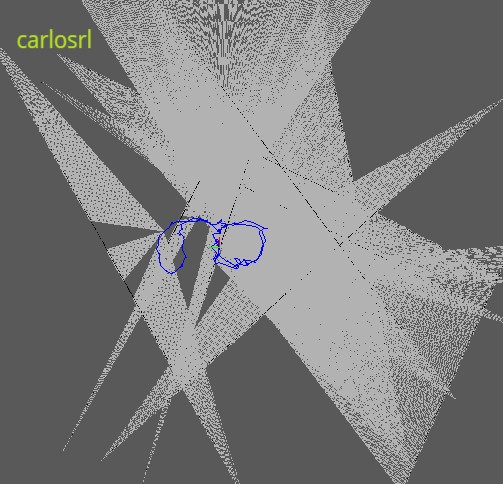
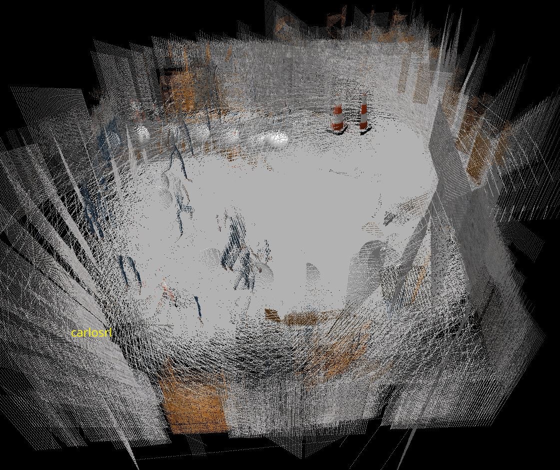
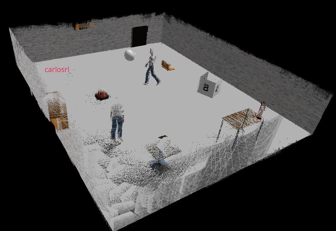
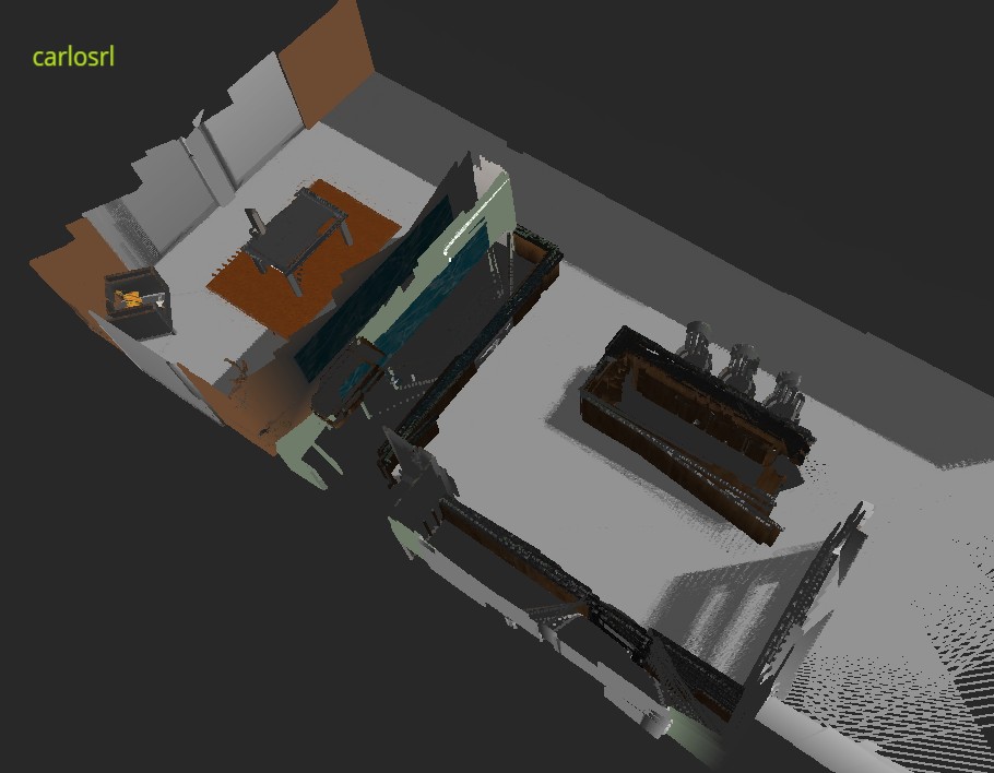
Now we have the 3D images for both worlds. It is clear that provided world has more features, as we can see reflected when we compare both worlds images.
Fig. 17 - 3D image with no optimization for created env.
Fig. 18 - 3D image with optimization for created env.
Fig. 19 - 3D image with no optimization for provided env.
Fig. 20 - 3D image with optimization for provided env.
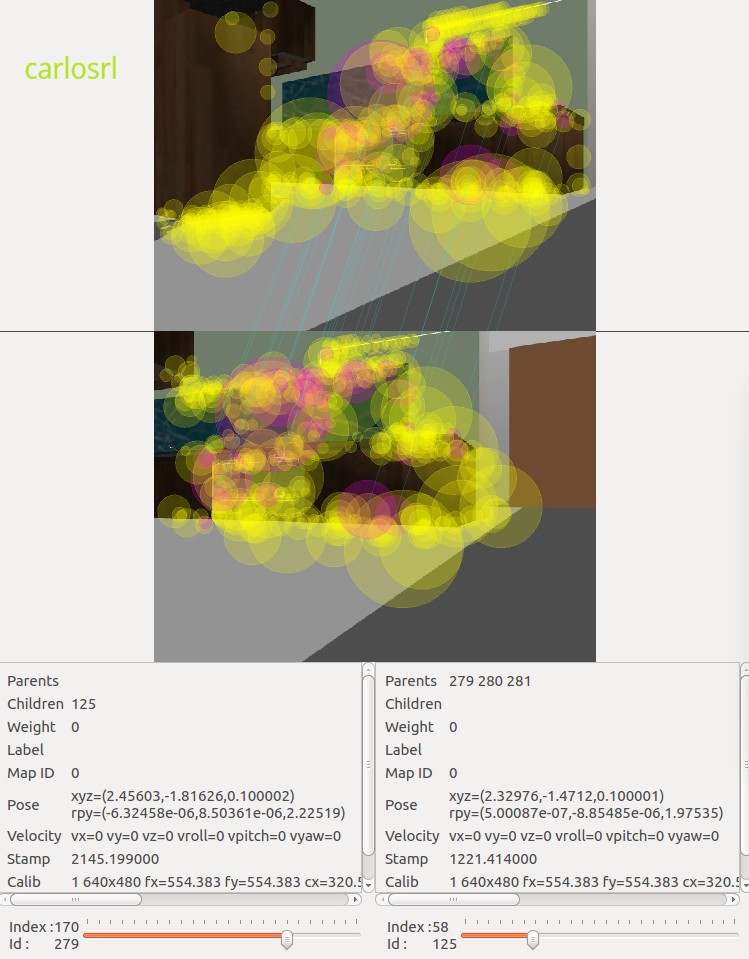
Then when we compare the mathing features, again the provided world has much more features than the created one.
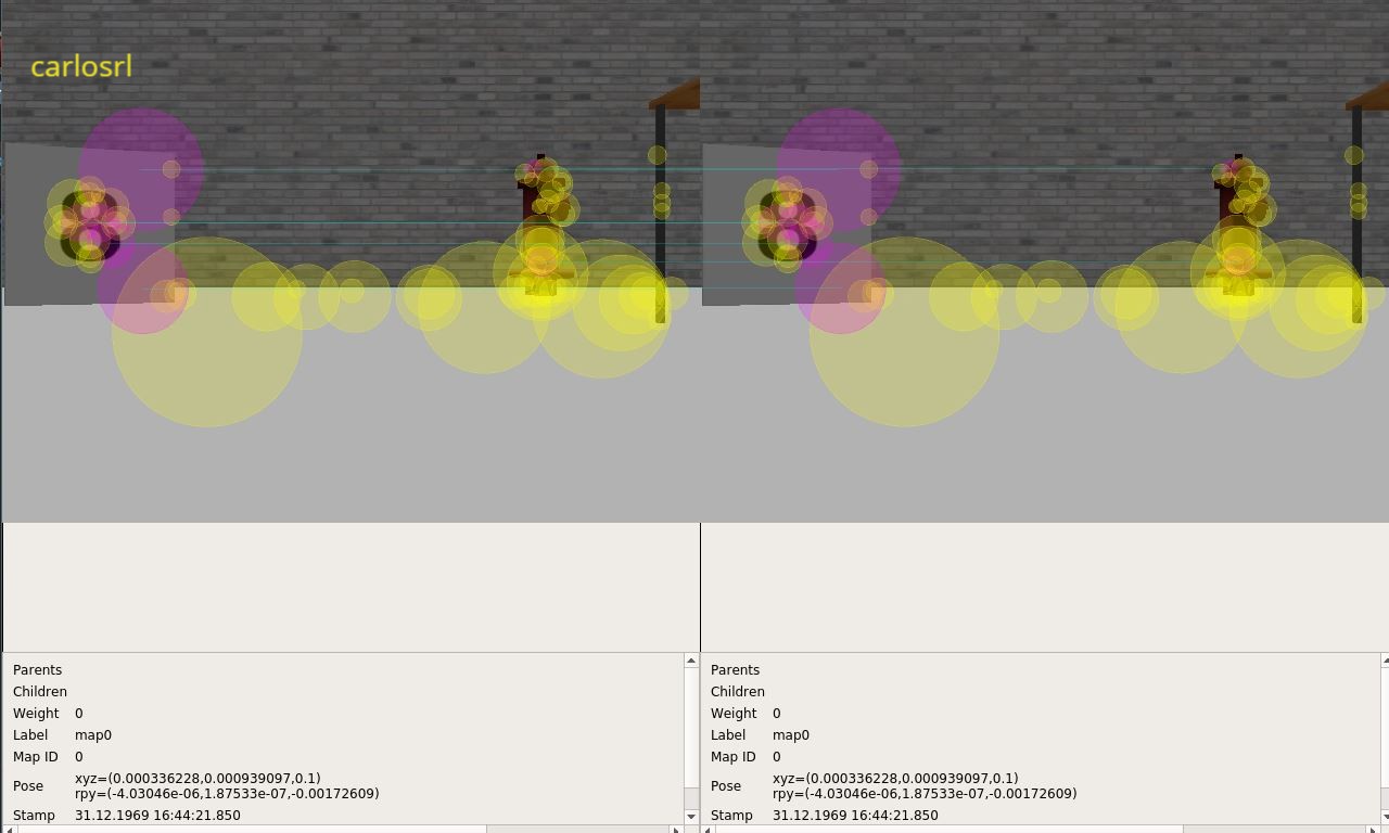
Fig. 21 - The image shows mathing features
Fig. 22 - The image shows mathing features
The figures 21 and 22 shows when mathing features are found in both worlds and how one is reacher in features than the other.
Thanks to Jetson TX2 that has computational resources sufficent to process the provided world. At first I tried to use the VM environment but it was unable to process the provided world. Moving to TX2 was the solution to finish this project.
The Fig. 21 and 22 shows the Bag-of-Words in action. A feature is a very specific characteristic of the image like a patch with complex texture or a corner or edge. For each feature a unique descriptor is associated to it. While new features are being located, the dictionary is searched loocking for matches that are represented by the lines in the image.
We can see that as more features in the environment, more matching lines we will see in the graphic.
The optimization applied to 2D and 3D maps seems to be very effective once that we can clearly identify the objects in optimized maps which does not occur when we see maps not optimized. But here we can see that this process is less effective when the enrironment has a high number of features as we can see in Fig. 19 and 20 where there is no big differences.
The RTAB-Map showed to see a heavy package in relation to computational resouce.
As commented in the begining of this document, the idea is to apply this process to a reaal robot.
If we consider apply this project to a drone, due to high computational tasks, we need take care about the battery size that can be consumed quickly if not well dimensioned.
